Using TREX to process Hyytiälä sap flow data
TREX Workflow
1. Background
The package TREX (tree sapflow extractor) provides functionalities for thermal dissipation sap flow data pre- and post-processing.
More specifically, raw sap flow data (expressed as temperature or voltage differences) can be:
- visually inspected and outliers can be identified and removed (manual and automatic detection) using
datacleanr, - zero-flow conditions can be derived using a wealth of well-established approaches,
- sap flow rates can be estimated using either literature- or user-specific calibration parameters for the thermal dissipation method,
- uncertainty of sap flow estimates stemming from parameter choices can be assessed by means of global sensitivity and uncertainty analysis,
- tree eco-physiologial responses to environmental drivers can be derived (e.g., crown conductance vs. vapor pressure deficit relations).
For more details, visit the dedicated
TREX website or the
manuscript.
2. Set-up Steps
# install if necessary
packages <- (c("remotes","zoo","lubridate","shiny","plotly"))
install.packages(setdiff(packages, rownames(installed.packages())))
remotes::install_github("the-Hull/TREX")
library(TREX)


# to get a full list of available functionalities check
#?TREX

library(zoo) # work with time series objects
library(lubridate) # work with date formats

# helper functions
left <-  function(string, char){substr(string, 1,char)}
right <-  function (string, char){substr(string,nchar(string)-(char-1),nchar(string))}
3. Data preparation
Import data
Sap flow time series and, if available, concurrently recorded meteorological data should be provided as input. Find an example data set to download and place in your current working directory here, or use the code below to download it directly.
# set you working directory on the correct path!
# click: Session -> Select Working Directory -> Choose Directory; or set using setwd()

url <- "https://raw.githubusercontent.com/deep-org/workshop_data/master/esa-workshop2021/sapflow_cleaned.Rds"
download.file(url, destfile = "sapflow_cleaned.Rds", method = "curl")

# import table cleaned with datacleanr
sensor<-readRDS("sapflow_cleaned.Rds")
head(sensor)
##             timestamp                          sensor value
## 1 2015-01-01 00:00:00 sapflux_density_birch_Jennib_HD    NA
## 2 2015-01-01 00:10:00 sapflux_density_birch_Jennib_HD    NA
## 3 2015-01-01 00:20:00 sapflux_density_birch_Jennib_HD    NA
## 4 2015-01-01 00:30:00 sapflux_density_birch_Jennib_HD    NA
## 5 2015-01-01 00:40:00 sapflux_density_birch_Jennib_HD    NA
## 6 2015-01-01 00:50:00 sapflux_density_birch_Jennib_HD    NA
unique(sensor$sensor)
## [1] "sapflux_density_birch_Jennib_HD" "sapflux_density_pine_Penttib_HD"
## [3] "sapflux_density_pine_Sylvib_HD"

# the code runs for individual trees, so we select the tree Pinus Sylvestris, i.e., 'sapflux_density_pine_Sylvib_HD'
sel_sensor<-sensor[which(sensor$sensor=="sapflux_density_pine_Sylvib_HD" ),]
# for the package we only need to timestamp and value
sel_sensor<-as.data.frame(sel_sensor)[,c("timestamp","value")]

# show the input data
plot(value~timestamp,data=sel_sensor,type="l")
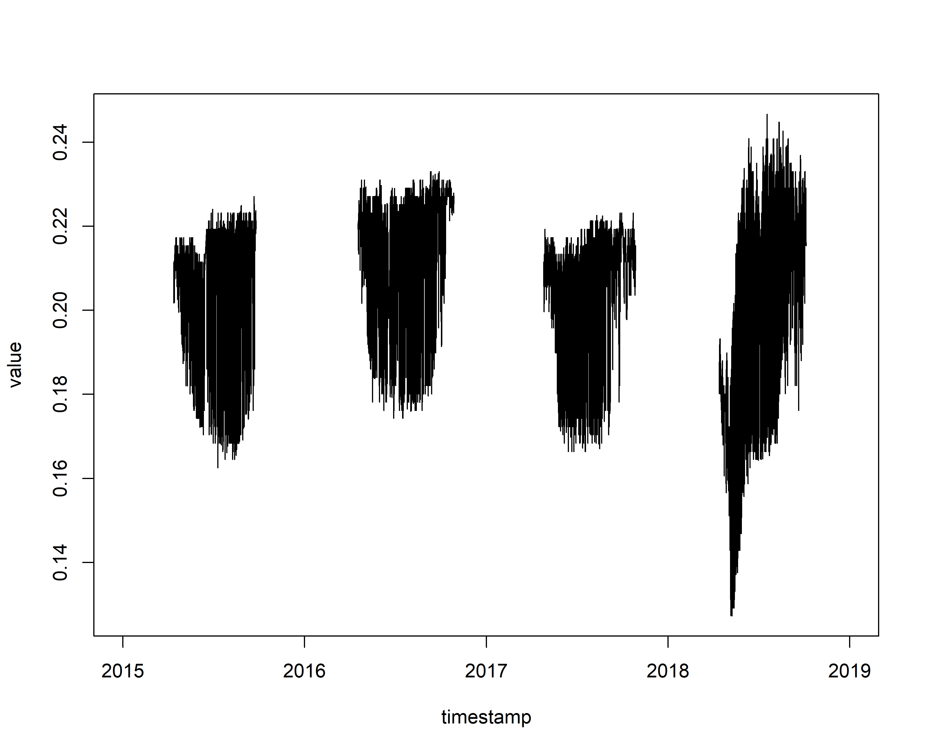
We can see from the data that there is a sensor drift in the \(\Delta V\) values (normally ranging between approximately 0.15 and 0.6) in the beginning of 2018. This could impact our final results. There are ways of correcting for such drifts, but for simplicity we ignore this issue. Now the data is ready for processing.
Create TREX-compatible objects and clip the same time period
The package includes functions for checking the consistency in the imported data (e.g., regular time steps in the time series objects, time zone and class of the time stamps).
# see help pages for the following functions (they take some time as they perform multiple internal checks)
?is.trex
## starting httpd help server ... done


sensor_raw_10min <- is.trex(sel_sensor,
                           tz="UTC",
                           time.format="%Y-%m-%d %H:%M:%S",
                           solar.time=F,
                           ref.add=FALSE,
                           df=FALSE,
                           tz.force=FALSE)
head(sensor_raw_10min)
## 2015-01-01 00:00:00 2015-01-01 00:10:00 2015-01-01 00:20:00 2015-01-01 00:30:00
##                  NA                  NA                  NA                  NA
## 2015-01-01 00:40:00 2015-01-01 00:50:00
##                  NA                  NA

# now that the data has been checked, we can adjust the start and the end time of the time series or alter the temporal resolution
?dt.steps
sensor_raw_1h <- dt.steps(input=sensor_raw_10min,
                         start = "2015-04-01 00:00:00",
                         end = "2018-10-31 23:30:00",
                         time.int=60, # here we define an hourly time resolution
                         max.gap=120, # here we define that linear interpolations are allowed for two hour to fill gaps
                         decimals=10,
                         df=FALSE)
plot(sensor_raw_1h, main="hourly raw sap flow data (mV)")
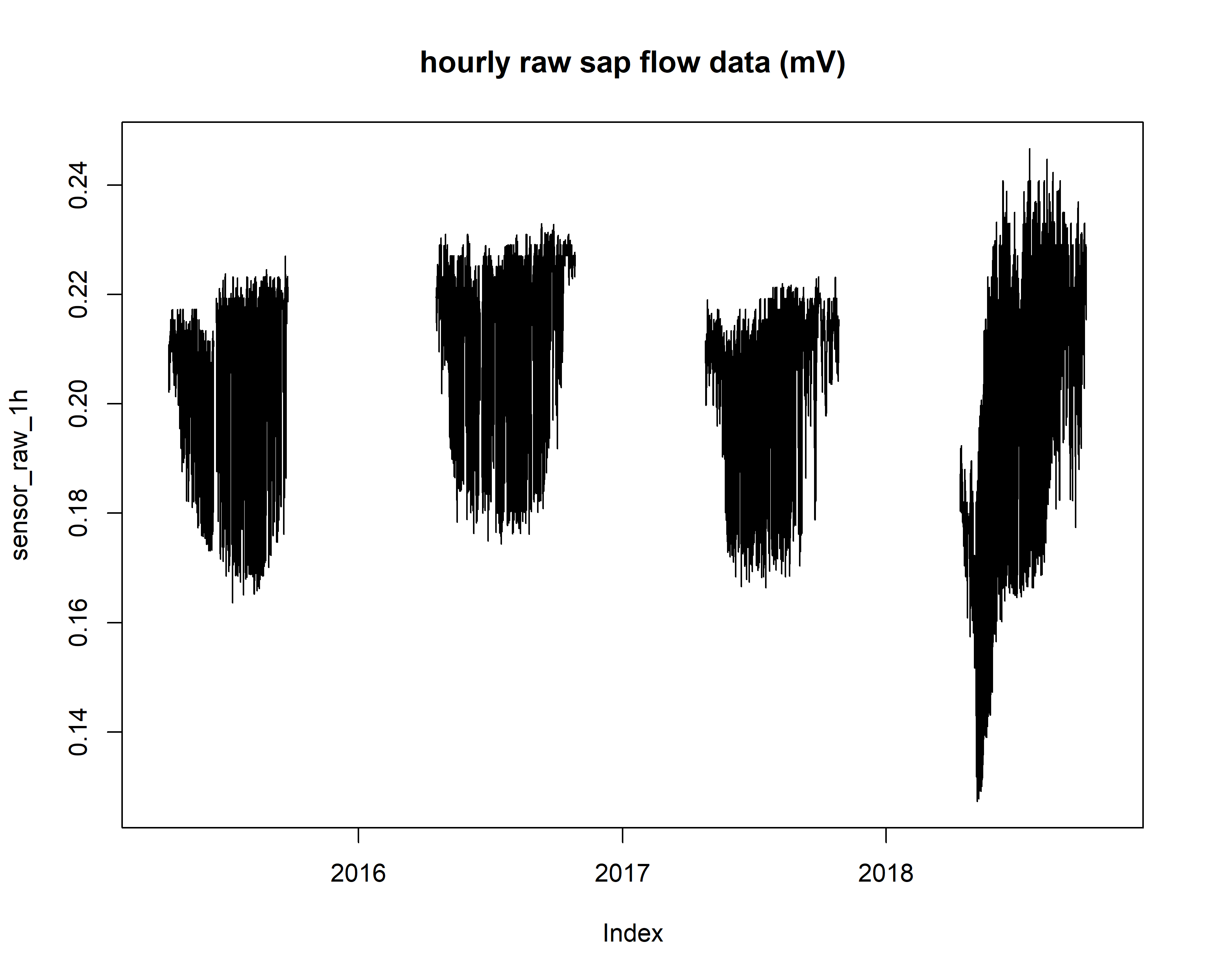
Now that the data has been checked by the internal TREX functions, multiple steps need to be taken to convert \(\Delta V\) values to sap flux density.
First we need to establish zero-flow conditions (which typically happen at night).
4. Estimate zero-flow conditions (DTmax)
# see help page for a detailed description
?tdm_dt.max
output.max <- tdm_dt.max(sensor_raw_1h,
methods = c("dr"), # for simplicity we use the double regression method (see help)
det.pd = TRUE,
interpolate = FALSE,
max.days = 5, # we select a 5 days window over which the zero flow conditions are considered
df = FALSE
)
# the structure of the output files is quite complex
str(output.max)
## List of 17
## $ max.pd :'zoo' series from 2015-04-01 to 2018-10-31 23:00:00
## Data: num [1:31440] NA NA NA NA NA NA NA NA NA NA ...
## Index: POSIXct[1:31440], format: "2015-04-01 00:00:00" "2015-04-01 01:00:00" ...
## $ max.mw : logi NA
## $ max.dr :'zoo' series from 2015-04-01 to 2018-10-31 23:00:00
## Data: num [1:31440] 0.215 0.215 0.215 0.215 0.215 ...
## Index: POSIXct[1:31440], format: "2015-04-01 00:00:00" "2015-04-01 01:00:00" ...
## $ max.ed : logi NA
## $ daily_max.pd:'zoo' series from 2015-04-01 to 2018-11-01
## Data: num [1:1311] NA NA NA NA NA NA NA NA NA NA ...
## Index: Date[1:1311], format: "2015-04-01" "2015-04-02" ...
## $ daily_max.mw: logi NA
## $ daily_max.dr:'zoo' series from 2015-04-01 to 2018-11-01
## Data: num [1:1311] 0.215 0.215 0.215 0.215 0.215 ...
## Index: Date[1:1311], format: "2015-04-01" "2015-04-02" ...
## $ daily_max.ed: logi NA
## $ all.pd :'zoo' series from 2015-04-01 to 2018-10-31 23:00:00
## Data: num [1:31440] NA NA NA NA NA NA NA NA NA NA ...
## Index: POSIXct[1:31440], format: "2015-04-01 00:00:00" "2015-04-01 01:00:00" ...
## $ all.ed : logi NA
## $ input :'zoo' series from 2015-04-01 to 2018-10-31 23:00:00
## Data: num [1:31440] NA NA NA NA NA NA NA NA NA NA ...
## Index: POSIXct[1:31440], format: "2015-04-01 00:00:00" "2015-04-01 01:00:00" ...
## $ ed.criteria : logi NA
## $ methods : chr "dr"
## $ k.pd :'zoo' series from 2015-04-01 to 2018-10-31 23:00:00
## Data: num [1:31440] NA NA NA NA NA NA NA NA NA NA ...
## Index: POSIXct[1:31440], format: "2015-04-01 00:00:00" "2015-04-01 01:00:00" ...
## $ k.mw : logi NA
## $ k.dr :'zoo' series from 2015-04-01 to 2018-10-31 23:00:00
## Data: num [1:31440] NA NA NA NA NA NA NA NA NA NA ...
## Index: POSIXct[1:31440], format: "2015-04-01 00:00:00" "2015-04-01 01:00:00" ...
## $ k.ed : logi NA
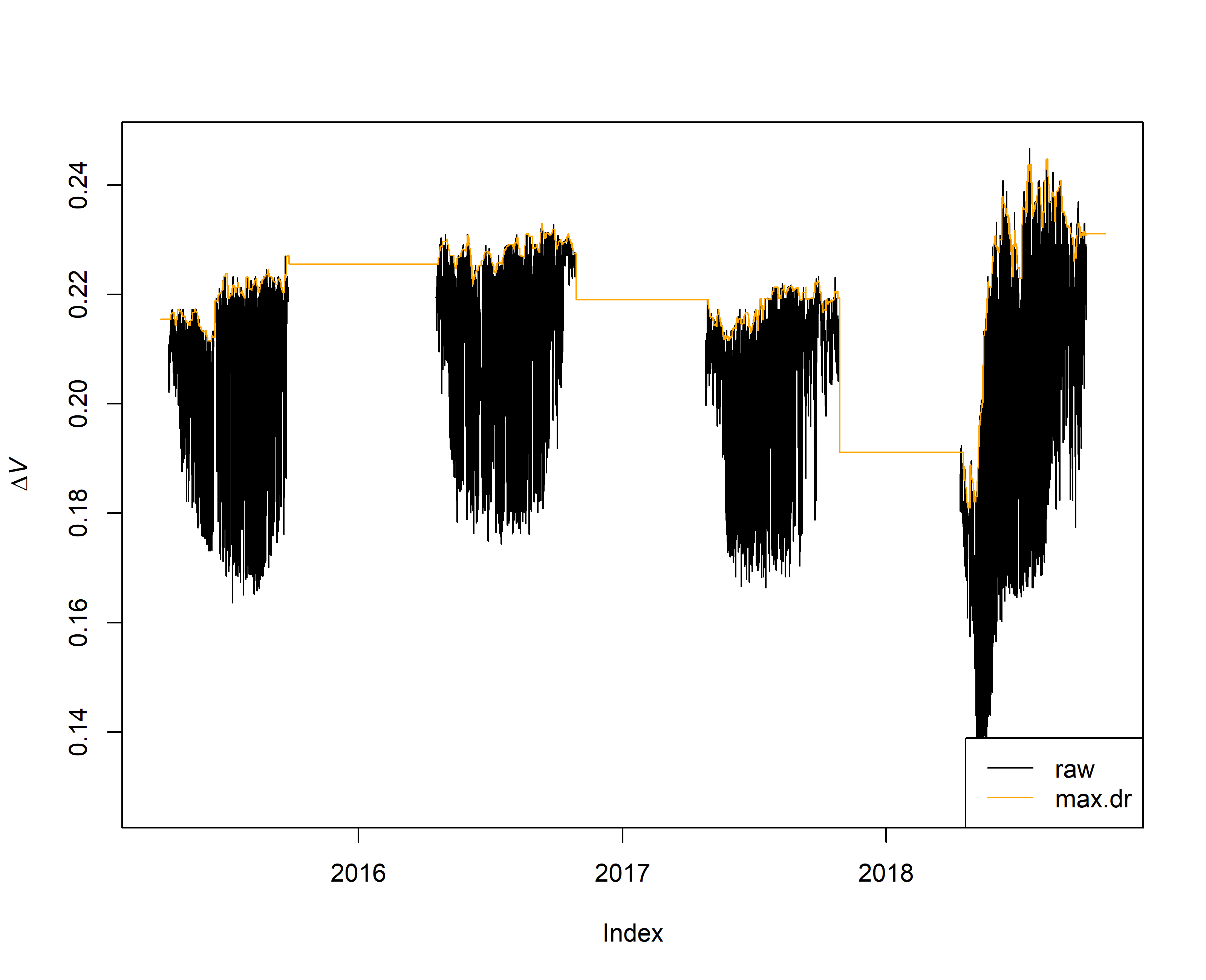
# however one can visualize what the code did by generating the following plot
{plot(output.max$input, ylab = expression(Delta*italic("V")))
lines(output.max$max.dr, col = "orange")
legend("bottomright", c("raw", "max.dr"),
lty = 1, col = c("black","orange") )
}
# for visualizing, clip a single month (July, 2016)
{plot(window(output.max$input, start="2015-07-15 00:00:00", end="2015-07-30 23:30:00"), ylab = expression(Delta*italic("V")))
lines(window(output.max$max.dr, start="2015-07-15 00:00:00", end="2015-07-30 23:30:00"), col = "orange")
legend("bottomright", c("raw",  "max.dr"),
       lty = 1, col = c("black","orange"))
}

The zero-flow condition values have been established and these will add in converting the raw \(\Delta V\) value to K.
K can be used to calculate sap flux density.
K is close to 0 when the raw data is close to the zero-flow condition value (orange lines in the previous plots).
A high proportional difference between the raw line and zero-flow conditions translates to high sap flow.
5. Correction of sensor artifacts
Apply heartwood correction (if needed)
# The sapwood depth of the selected tree is 4.3 cm, and the probe length 4 cm, so no heartwood correction needs to be applied

# see help page for a detailed description
#?tdm_hw.cor

#SFD_cor = tdm_hw.cor(output.max,probe.length=40,
#                     sapwood.thickness= 43,
#                     df=F)
As no heartwood correction is needed we can now calculate the K values and convert these values to sap flux density (using existing calibration parameters).
6. Calculate sap flux density
# see help page for a detailed description
?tdm_cal.sfd

# let look at the species present within the calibration database
unique(cal.data$Species)
##  [1] "Vitis vinifera"                 "Malus domestica"
##  [3] "Quercus sp."                    "Castanea sativa"
##  [5] "Macaranga hypoleuca"            "Macaranga pearsonii"
##  [7] "Abies concolor"                 "Acer pseudoplatanus"
##  [9] "Fagus sylvatica"                "Tilia cordata"
## [11] "Acer campestre"                 "Populus nigra"
## [13] "Pseudotzuga menziesii"          "Pinus nigra"
## [15] "Quercus pedunculata"            "Hyeronima alchorneoides"
## [17] "Crataegus monogina"             "Musa spp."
## [19] "Mangifera indica"               "Carica papaya"
## [21] "Peltophorum dubium"             "Prunus persica"
## [23] "Eucalyptus globulus"            "Eucalyptus nitens x globulus"
## [25] "Populus sp"                     "Phoenix datylifera"
## [27] "Pyrus serotina"                 "Liquidambar styraciflua"
## [29] "Populus deltoides"              "Quercus alba"
## [31] "Ulmus americana"                "Pinus echinata"
## [33] "Pinus taeda"                    "Eucalyptus grandis x urophylla"
## [35] "Larix decidua"                  "Picea abies"
## [37] "Fagus grandifolia"

# as there is no data for Scots pine we will use the average calibration found for coniferous species
SFD_damp<-output.max
output.data <- tdm_cal.sfd(SFD_damp,
                          make.plot=T,
                          df=FALSE,
                          wood = "Coniferous")
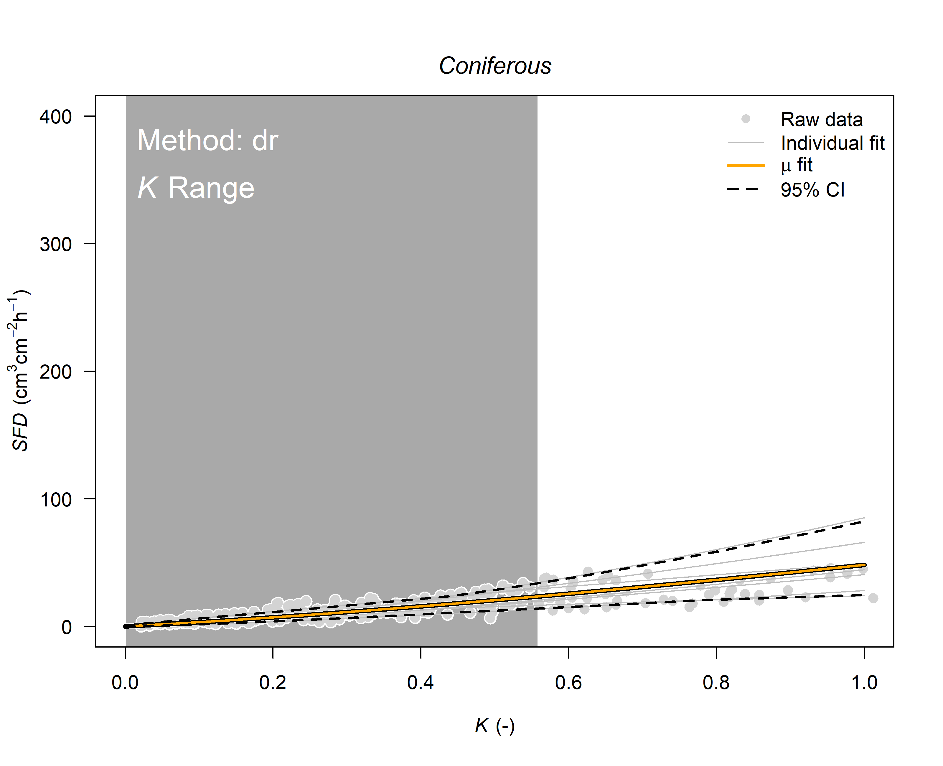
Now that we have calculated the sap flux density (SFD in \(cm^3 cm^{-2} h^{-1}\)) we need to inspect the data.
# extract the sfd data from the data file
sfd_data<-output.data$sfd.dr$sfd

# plotting the data
plot(sfd_data,ylab=expression("SFD ("*cm^3*" water "*cm^-2*" sapwood "*h^-1*")"))
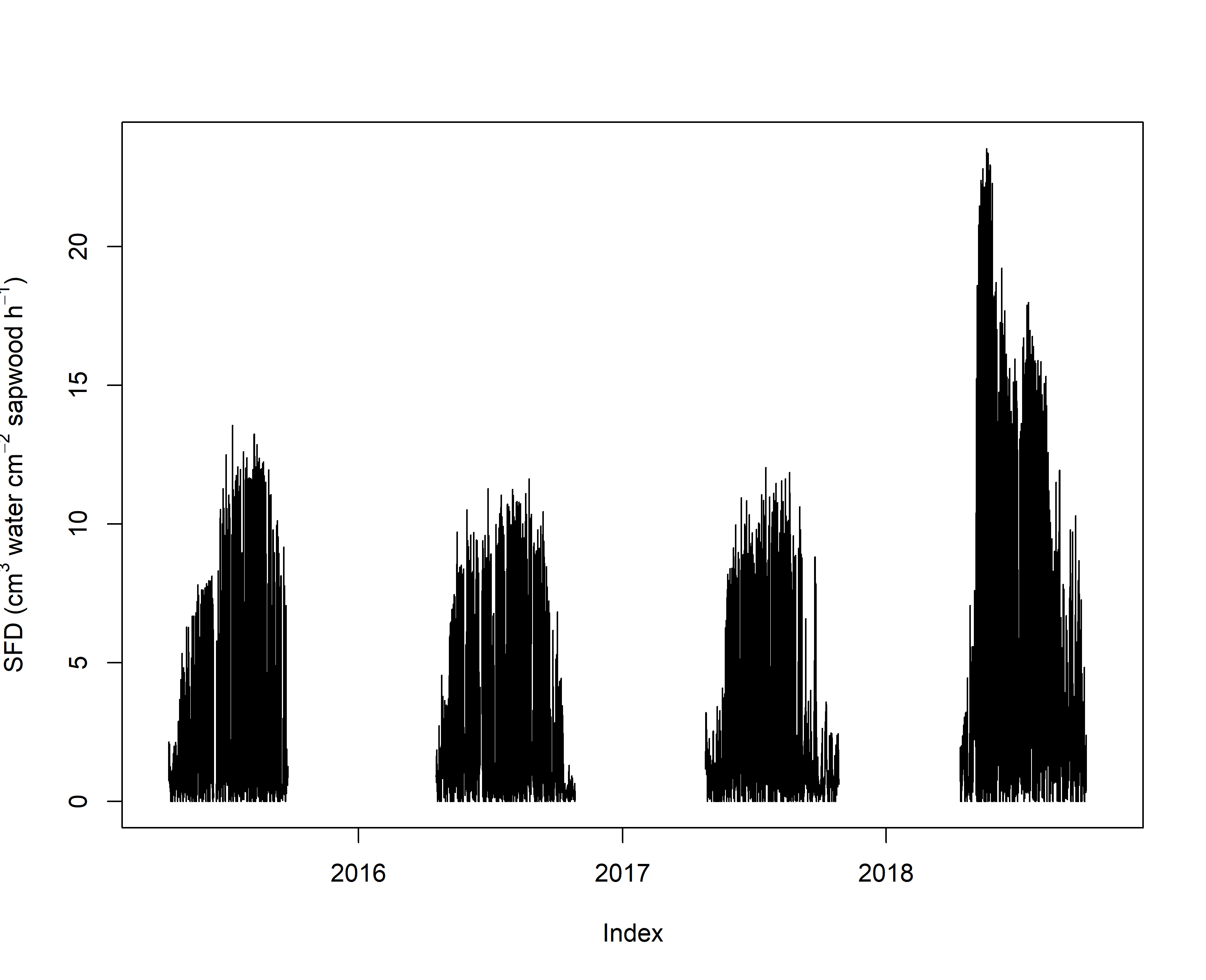
From this plot it is clear that the sensor drift in 2018 provided high an likely unrealistic values. A such we focus our analyses on 2015, 2016 and 2017. Be are aware that there are methods to deal with such drifts.
# extract the sfd data from the data file
sfd_final<-window(sfd_data,start= as.POSIXct("2015-01-01 00:00:00",format="%Y-%m-%d %H:%M:%S",tz="UTC"),
                end= as.POSIXct("2017-12-31 00:00:00",format="%Y-%m-%d %H:%M:%S",tz="UTC"))
Assignment:
Sap flux density data is highly relevant as it can provide information on both the maximum transpiration rates per unit sapwood area as the total water use per year. For context, this tree has a diameter of 20.6 cm, a bark thickness of 1.3 cm and a sapwood thickness of 4.3 cm. With this information we can calculate the daily transpiration rate per sapwood area and for the entire tree (by multiplying the sap flux density value by the sapwood area). Using the sap flow data one can ask:
- What is the maximum daily transpiration per unit sapwood area for each year?
- What is the total amount of water (in liters) this tree used per day?
- What is the total amount of water the tree used over these three years?
To answer these questions please generate a barplot illustrating the maximum daily sap flux density and make a scatter plot to show the daily water use.
Hint: As the data is in a hourly time-step and provide the flux per hour, one can sum the values for each day to obtain the daily flux rate:
example <- aggregate(data,order.by=as.Date(index(data)),sum,na.rm=T)
Also, see https://doi.org/10.1093/treephys/18.8-9.499 for a review on total daily water use in trees.
Solution
# prepare the data
sfd_daily<-aggregate(sfd_final,by=as.Date(index(sfd_final)),sum,na.rm=T)
#plot(sfd_daily, ylab=expression("water ("*g*" "*cm^-2*" "*d^-1*")"))
sfd_annual<-aggregate(sfd_daily,by=list(left(as.Date(index(sfd_daily)),4)),max,na.rm=T)
input<-data.frame(year=as.factor(index(sfd_annual)),max_daily_sfd=as.numeric(sfd_annual))
barplot(max_daily_sfd~year,data=input,beside=T)
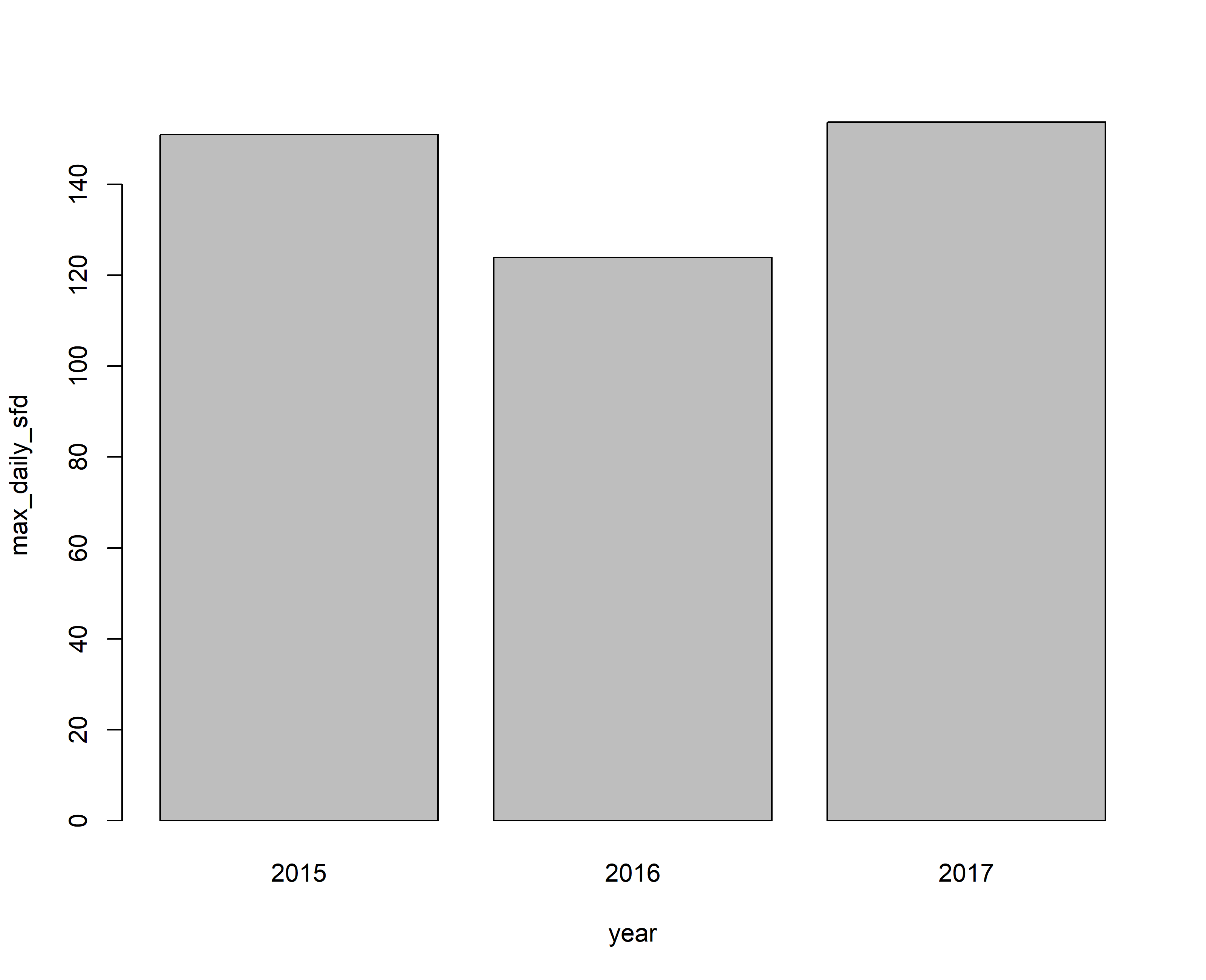
#Question 1. In 2015 the tree had a maximum sap flux density of 151 g cm-2 d-1, followed by 2017 with 154 g cm-2 d-1 and 124 g cm-2 d-1 for 2016.

# calculating the sap wood area
rad_xylem<-(20.6-(1.3*2))/2
rad_heartwood<-rad_xylem-4.3
sw_area<-pi*(rad_xylem^2)-pi*(rad_heartwood^2)
sf_daily<-sfd_daily*sw_area*0.001
plot(sf_daily,ylab=expression("Water (l "*d^-1*")"))
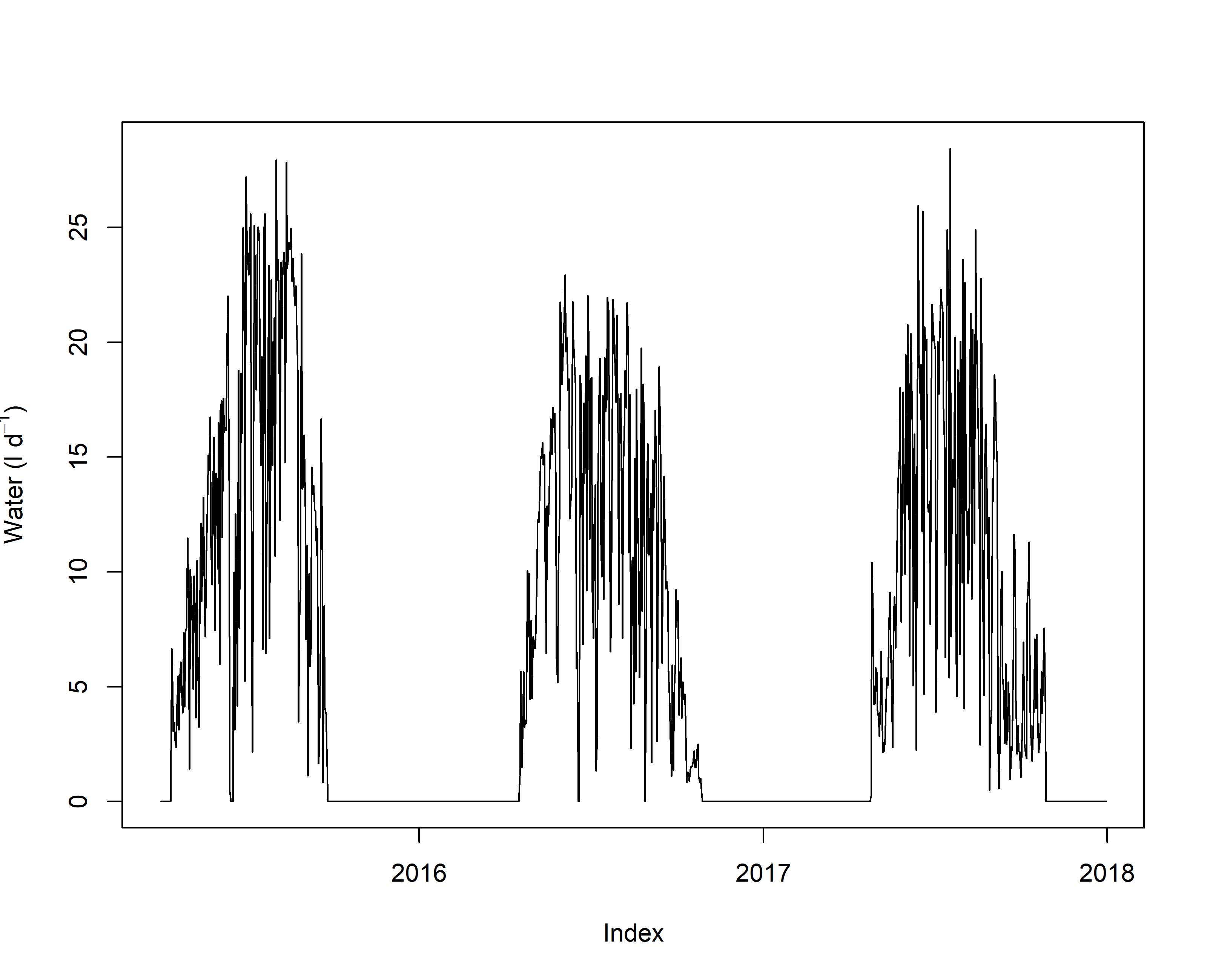
# Question 2: The daily water use appears to be around 15 liters of water per day which appears realistic when comparing this to other conifer species.

sf_annual<-aggregate(sf_daily,by=list(left(as.Date(index(sf_daily)),4)),sum,na.rm=T)
print(paste0("Water use from 2015-2017: ",round(sum(sf_annual),0)," liters of water"))
## [1] "Water use from 2015-2017: 6278 liters of water"

# Question 3: To total amount fo water used by these trees over these three years is over 6000 liters of water.
7. Estimate uncertainties with a global sensitivity/uncertainty analysis
The implemented methods for the global sensitivity and uncertainty analysis give an indication on the contribution of individual variables/constants to variability of final outputs. However, they are computational demanding and thus we have selected a sub-period of few months for illustration purposes. For details on this method please refer to this section in our open-access article.
# see help page for a detailed description
#?tdm_uncertain
set.seed(1234)
output <- tdm_uncertain(window(sensor_raw_1h,
                              start = "2015-04-01 00:00:00",
                              end = "2015-09-01 00:00:00"),
                       probe.length=20,
                       method="pd",
                       n=2000,
                       sw.cor=25,
                       sw.sd=16,
                       log.a_mu=output.data$out.param$log.a_mu,
                       log.a_sd=output.data$out.param$log.a_sd,
                       b_mu=output.data$out.param$b_mu,
                       b_sd=output.data$out.param$b_sd,
                       make.plot=TRUE)

8. Using TREX
For use in publication, the reference is:
citation("TREX")
##
## To cite TREX in publications use:
##
##   Peters, R. L., Pappas, C., Hurley, A. G., Poyatos, R., Flo, V.,
##   Zweifel, R., Goossens, W., & Steppe, K. (2021). Assimilate, process
##   and analyse thermal dissipation sap flow data using the TREX r
##   package. Methods in Ecology and Evolution, 12(2), 342–350.
##   https://doi.org/10.1111/2041-210X.13524
##
## A BibTeX entry for LaTeX users is
##
##   @Article{,
##     title = {Assimilate, Process and Analyse Thermal Dissipation Sap Flow Data Using the {{TREX}} R Package},
##     author = {Richard L Peters and Christoforos Pappas and Alexander G Hurley and Rafael Poyatos and Victor Flo and Roman Zweifel and Willem Goossens and Kathy Steppe},
##     journal = {Methods in Ecology and Evolution},
##     year = {2021},
##     volume = {12},
##     number = {2},
##     pages = {342--350},
##     url = {https://besjournals.onlinelibrary.wiley.com/doi/abs/10.1111/2041-210X.13524},
##     doi = {10.1111/2041-210X.13524},
##     issn = {2041-210X},
##   }
9. References
- Peters, R. L., Pappas, C., Hurley, A. G., Poyatos, R., Flo, V., Zweifel, R., Goossens, W., & Steppe, K. (2021). Assimilate, process and analyse thermal dissipation sap flow data using the TREX r package. Methods in Ecology and Evolution, 12(2), 342–350. https://doi.org/10.1111/2041-210X.13524
- Richard Peters, Christoforos Pappas and Alexander Hurley (2020). TREX: TRree sap flow EXtractor. R package version 0.0.0.9000. https://the-hull.github.io/TREX/
10. Contact
For questions, please get in touch with Christoforos Pappas