Analysis Workflow
1. Background
The package TREX (tree sapflow extractor) provides functionalities for thermal dissipation sap flow data pre- and post-processing.
More specifically, raw sap flow data (expressed as temperature or voltage differences) can be:
- visually inspected and outliers can be identified and removed (manual and automatic detection),
- zero-flow conditions can be derived using a wealth of well-established approaches,
- sap flow rates can be estimated using either literature- or user-specific calibration parameters for the thermal dissipation method,
- uncertainty of sap flow estimates stemming from parameter choices can be assessed,
- tree ecophysiologial responses to environmental drivers can be derived (e.g., crown conductance vs vapor pressure deficit relations).
For more details, visit the dedicated
TREX website
2. Set-up Steps
# install if necessary
packages <- (c("remotes","zoo","lubridate","shiny","plotly"))
install.packages(setdiff(packages, rownames(installed.packages())))
remotes::install_github("the-Hull/TREX")
library(TREX)
# to get a full list of available functionalities check
#?TREX

library(zoo) # work with time series objects
library(lubridate) # work with date formats
library(shiny) # visual inspection and outlier detection
library(plotly) # interactive plots
3. Data preparation
Import data
Sap flow time series data and concurrently recorded meteorological data should be provided as input.
# URLs were the data are stored
vpd_url <- RCurl::getURL("https://raw.githubusercontent.com/deep-org/workshop_data/master/esa-workshop2020/Environmental%20data/Vapour_pressure_deficit%20(kPa).txt")
rad_url <- RCurl::getURL("https://raw.githubusercontent.com/deep-org/workshop_data/master/esa-workshop2020/Environmental%20data/Solar_radiance%20(W%20m-2).txt")
prc_url <- RCurl::getURL("https://raw.githubusercontent.com/deep-org/workshop_data/master/esa-workshop2020/Environmental%20data/Precipitation%20(mm).txt")

sensor_url <- RCurl::getURL("https://raw.githubusercontent.com/deep-org/workshop_data/master/esa-workshop2020/TDP%20data/N13Ad_S1_dV%20(mv).txt")

# VPD (15-min)
vpd <- read.table(text = vpd_url, header=T, sep="\t")
head(vpd)
##             Timestamp VPD
## 1 (10/19/06 16:15:00)  NA
## 2 (10/19/06 16:30:00)  NA
## 3 (10/19/06 16:45:00)  NA
## 4 (10/19/06 17:00:00)  NA
## 5 (10/19/06 17:15:00)  NA
## 6 (10/19/06 17:30:00)  NA

# solar radiation (15-min)
rad <- read.table(text = rad_url, header=T, sep="\t")
head(rad)
##             Timestamp    SR
## 1 (10/19/06 16:15:00) 83.33
## 2 (10/19/06 16:30:00) 58.67
## 3 (10/19/06 16:45:00) 58.67
## 4 (10/19/06 17:00:00) 30.33
## 5 (10/19/06 17:15:00) 18.33
## 6 (10/19/06 17:30:00)  5.00

# precipitation (daily)
prc <- read.table(text = prc_url, header=T, sep="\t")
head(prc)
##   Timestamp      Prec
## 1  01/01/06 2.9140029
## 2  02/01/06 1.4081558
## 3  03/01/06 0.0821319
## 4  04/01/06 0.0000000
## 5  05/01/06 0.0000000
## 6  06/01/06 0.0000000


# sap flow (15-min)
sensor <- read.table(text = sensor_url, header=T, sep="\t")
head(sensor)
##             Timestamp dV
## 1 (04/17/12 15:00:00) NA
## 2 (04/17/12 15:15:00) NA
## 3 (04/17/12 15:30:00) NA
## 4 (04/17/12 15:45:00) NA
## 5 (04/17/12 16:00:00) NA
## 6 (04/17/12 16:15:00) NA

# convert to data.frames with timestamp as 'date'
vpd <- data.frame(timestamp = mdy_hms(vpd$Timestamp, tz="GMT"), value = vpd$VPD)
rad <- data.frame(timestamp = mdy_hms(rad$Timestamp, tz="GMT"), value = rad$SR)
prc <- data.frame(timestamp = dmy(prc$Timestamp, tz="GMT"), value = prc$Prec)
sensor = data.frame(timestamp = mdy_hms(sensor$Timestamp, tz="GMT"), value = sensor$dV)
Create TREX-compatible objects and clip the same time period of sap flow and meteorological data
The package includes functions for checking the consistency in the imported data (e.g., regular time steps in the time series objects, time zone and class of the time stamps).
# see help pages for the following functions
#?is.trex
#?dt.steps
sensor_raw_15min <- is.trex(sensor,
tz="GMT",
time.format="%Y-%m-%d %H:%M:%S",
solar.time=T,
long.deg=7.7459,
ref.add=FALSE,
df=FALSE)
sensor_raw_1h <- dt.steps(input=sensor_raw_15min,
start = "2012-05-01 00:00:00",
end = "2015-10-31 23:30:00",
time.int=60,
max.gap=120,
decimals=10,
df=FALSE)
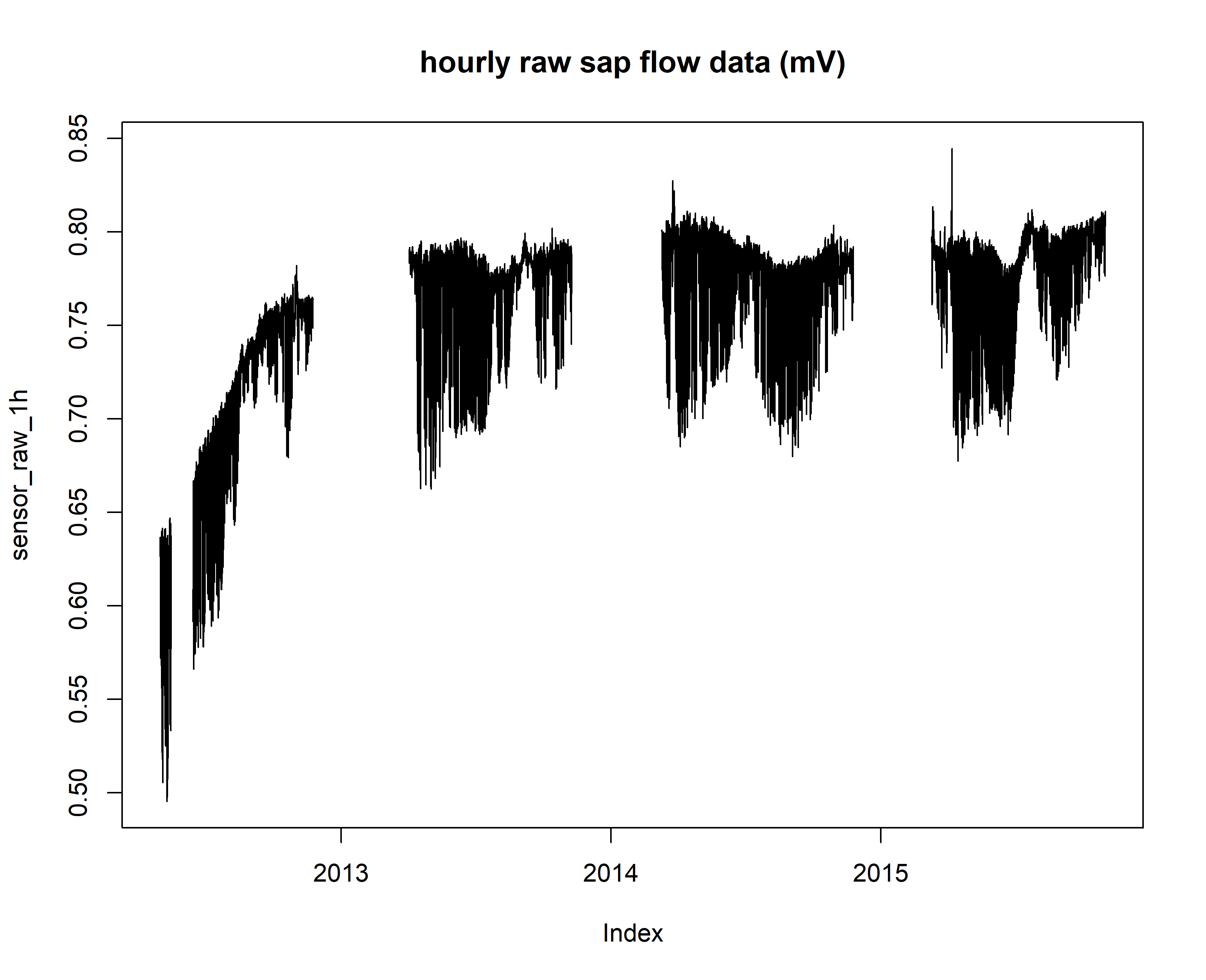
plot(sensor_raw_1h, main="hourly raw sap flow data (mV)")

# make a data.frame
sensor_raw_1h_df <- data.frame(timestamp = ymd_hms(index(sensor_raw_1h), tz="GMT"), value = coredata(sensor_raw_1h))
vpd_15min <- is.trex(vpd,
tz="GMT",
time.format="%Y-%m-%d %H:%M:%S",
solar.time=T,
long.deg=7.7459,
ref.add=FALSE,
df=FALSE)
# vpd data
vpd_1h <- dt.steps(input=vpd_15min,
start = "2012-05-01 00:00:00",
end = "2015-10-31 23:30:00",
time.int=60,
max.gap=120,
decimals=10,
df=FALSE)
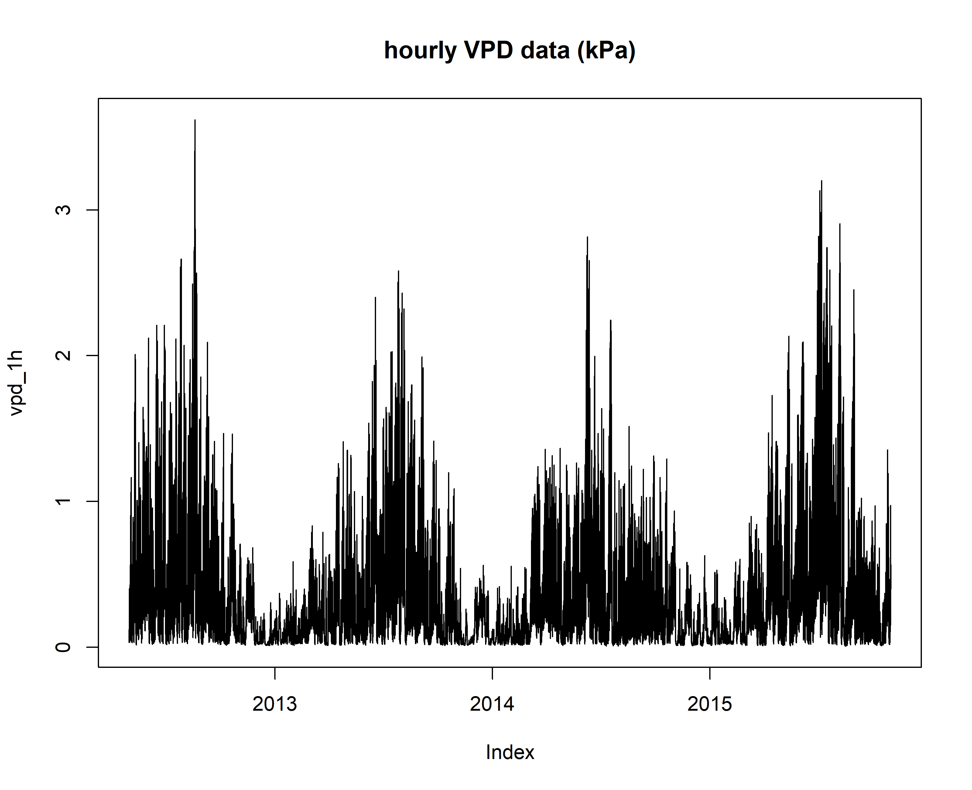
plot(vpd_1h, main="hourly VPD data (kPa)")
# radiation data
rad_15min <- is.trex(rad,
tz="GMT",
time.format="%Y-%m-%d %H:%M:%S",
solar.time=T,
long.deg=7.7459,
ref.add=FALSE,
df=FALSE)
rad_1h <- dt.steps(input=rad_15min,
start = "2012-05-01 00:00:00",
end = "2015-10-31 23:30:00",
time.int=60,
max.gap=120,
decimals=10,
df=FALSE)
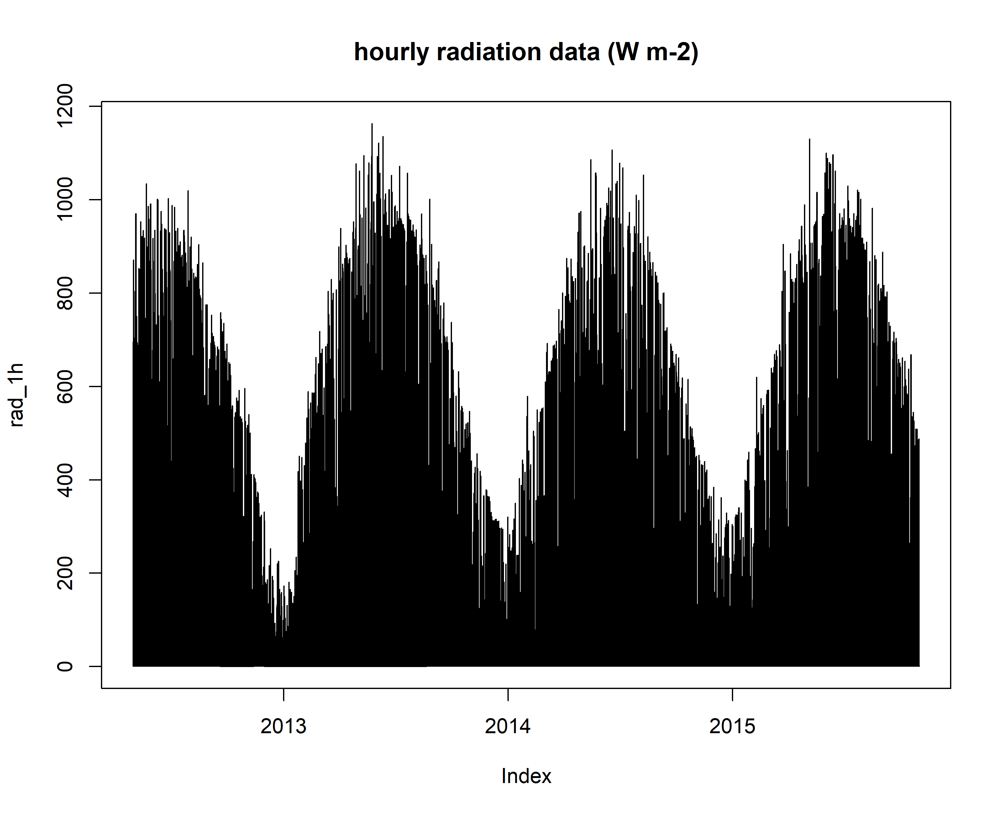
plot(rad_1h, main="hourly radiation data (W m-2)")
# precip data
prc_1day <- is.trex(prc,
tz="GMT",
time.format="%Y-%m-%d",
solar.time=T,
long.deg=7.7459,
ref.add=FALSE,
df=FALSE)
prc_1day <- window(prc_1day, start = "2012-05-01 00:00:00", end = "2015-10-31 23:30:00")
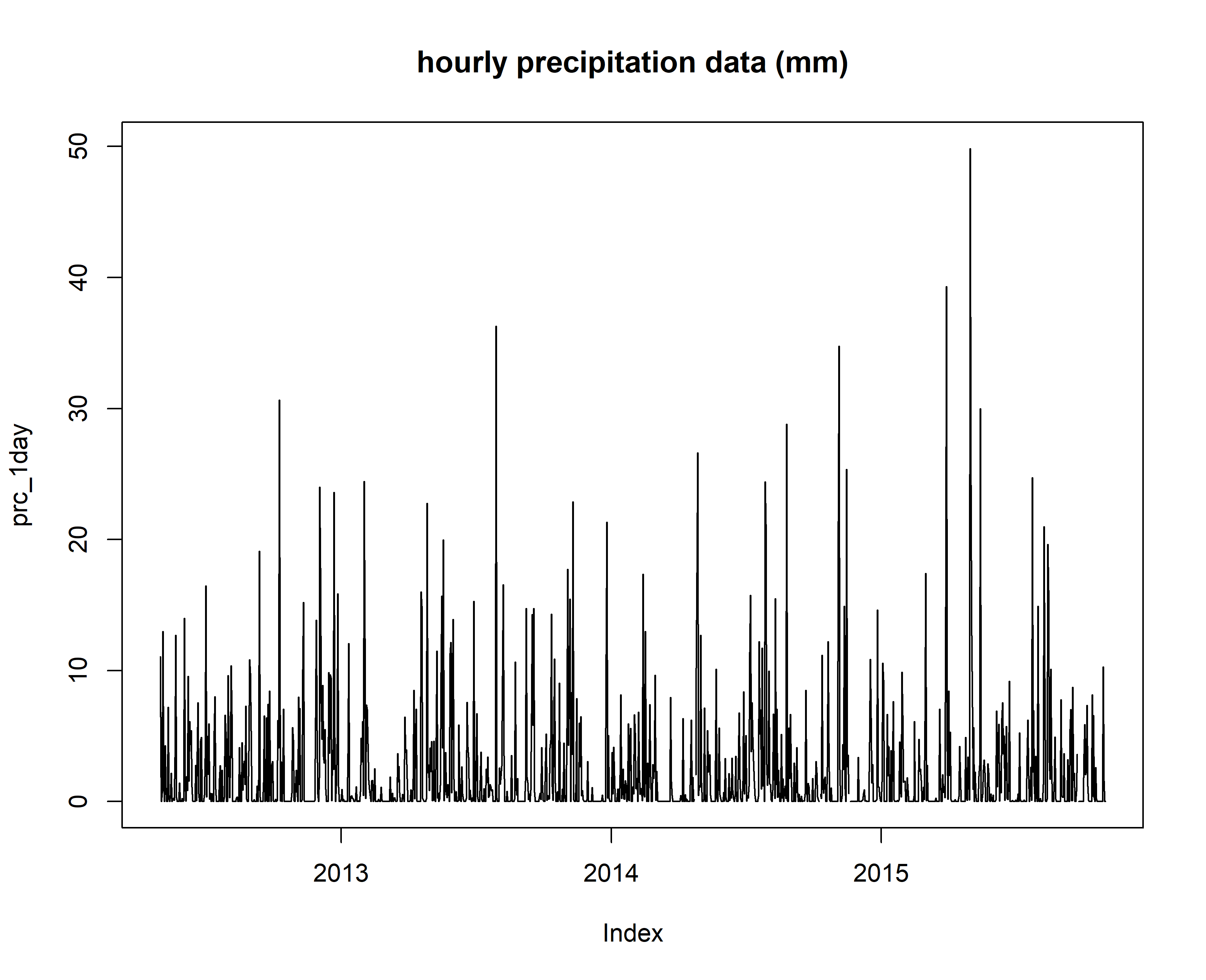
plot(prc_1day, main="hourly precipitation data (mm)")
Visual inspection of time series, outlier detection and removal
Note: the current version of outlier detection cannot handle large datasets (e.g., hourly data for several years) cause the interactive plots become slow. We suggest, if you have long time series that you would like to inspect, to split the time series in shorter time periods and run the following steps sequentially.
Here, we provide an illustration of the functionalities of the outlier() using couple of months of hourly sap flow data.
In action, the outlier function looks as follows:
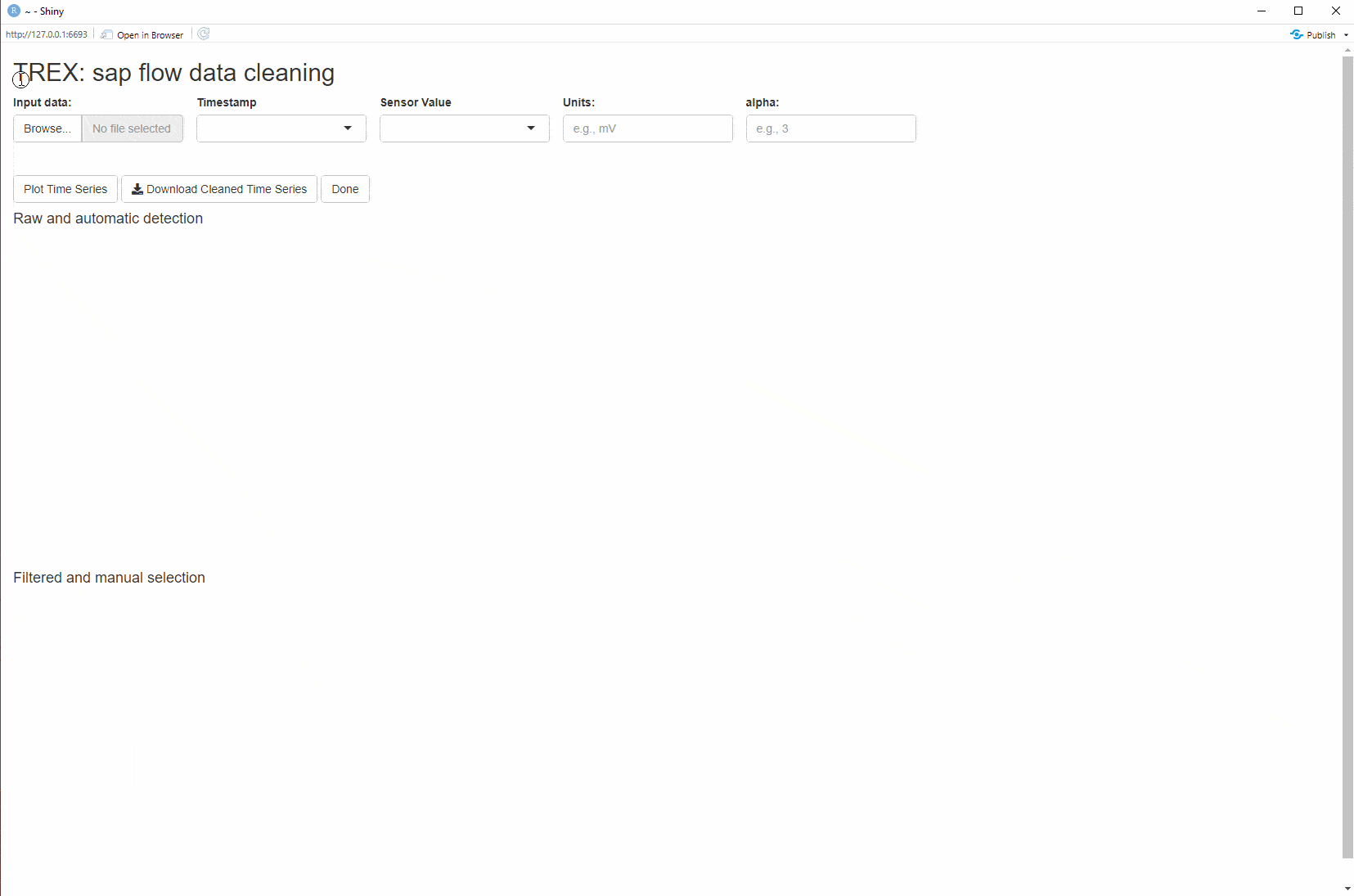 Figure: Application of the
 outlier() function to the example data set - note the interactive selection and deselection of observations considered outliers. The interactive app allows saving a list to disk with the original data set, the cleaned version, as well as subsets containing the automatic and the manual outlier selection.
# see help page for a detailed description
#?outlier()

# from a quick visual inspection of the hourly time sap flow time series data, we see that there are few irregularities, and potential outliers at the beginning of the 2015 growing season

plot(sensor_raw_1h, main="hourly raw sap flow data (mV)")
# zoom-in to a shorter time period
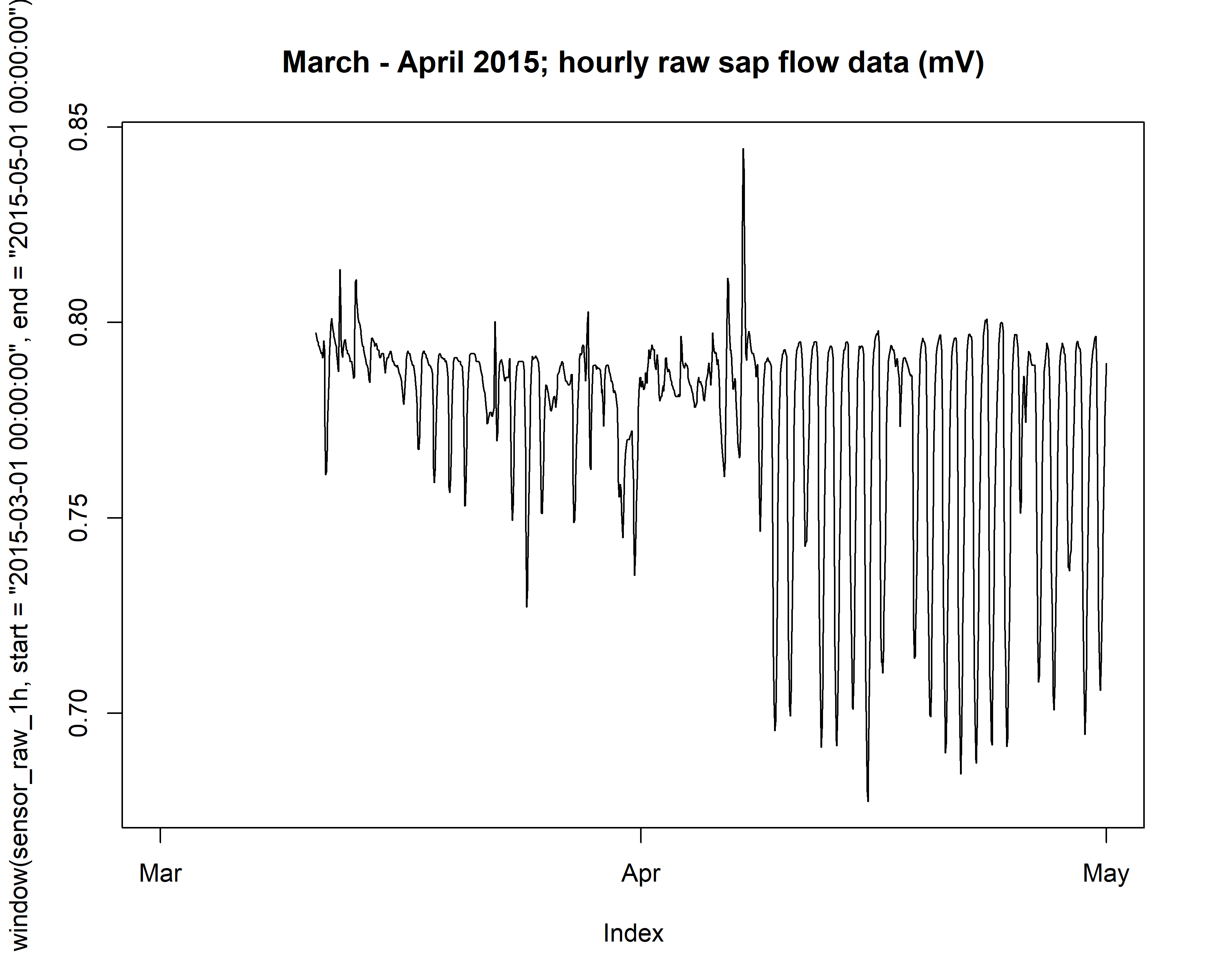
plot(window(sensor_raw_1h, start = "2015-03-01 00:00:00", end = "2015-05-01 00:00:00"), main="March - April 2015; hourly raw sap flow data (mV)")
# create an object with the period of interest, i.e., March - April 2015
tocheck <- window(sensor_raw_1h, start = "2015-03-01 00:00:00", end = "2015-05-01 00:00:00")
# make a data.frame
tocheck_df <- data.frame(timestamp = ymd_hms(index(tocheck), tz="GMT"), value = coredata(tocheck))
# save an .RData
save(tocheck_df, file="tocheck.RData")
# call outlier() app and load the generated .RData file
#outlier()
# after inspecting the time series with the outlier() an .RDS file is exported with the 'outlier-free' data.
# load the 'tocheck_Cleaned.Rds' file
tocheck_Cleaned <- readRDS("tocheck_Cleaned.Rds")
tocheck_Cleaned <- tocheck_Cleaned$series_cleaned
summary(tocheck_Cleaned)
## timestamp value
## Min. :2015-03-01 00:00:00 Min. :0.6774
## 1st Qu.:2015-03-16 05:45:00 1st Qu.:0.7700
## Median :2015-03-31 10:30:00 Median :0.7864
## Mean :2015-03-31 11:50:37 Mean :0.7752
## 3rd Qu.:2015-04-15 19:15:00 3rd Qu.:0.7914
## Max. :2015-05-01 00:00:00 Max. :0.8113
## NA's :241
summary(sensor_raw_1h_df)
## timestamp value
## Min. :2012-05-01 00:00:00 Min. :0.495
## 1st Qu.:2013-03-16 17:45:00 1st Qu.:0.748
## Median :2014-01-30 11:30:00 Median :0.779
## Mean :2014-01-30 11:30:00 Mean :0.762
## 3rd Qu.:2014-12-16 05:15:00 3rd Qu.:0.789
## Max. :2015-10-31 23:00:00 Max. :0.845
## NA's :9307
# Merge the cleaned data with the complete 'sensor_raw_1h' time series
sensor_raw_1h_df_clean <- sensor_raw_1h_df
sensor_raw_1h_df_clean[(sensor_raw_1h_df_clean$timestamp >= "2015-03-01 00:00:00" & sensor_raw_1h_df_clean$timestamp <= "2015-05-01 00:00:00"),"value"] <- NA
sensor_raw_1h_df_clean[sensor_raw_1h_df_clean$timestamp %in% tocheck_Cleaned$timestamp, "value"] =tocheck_Cleaned$value
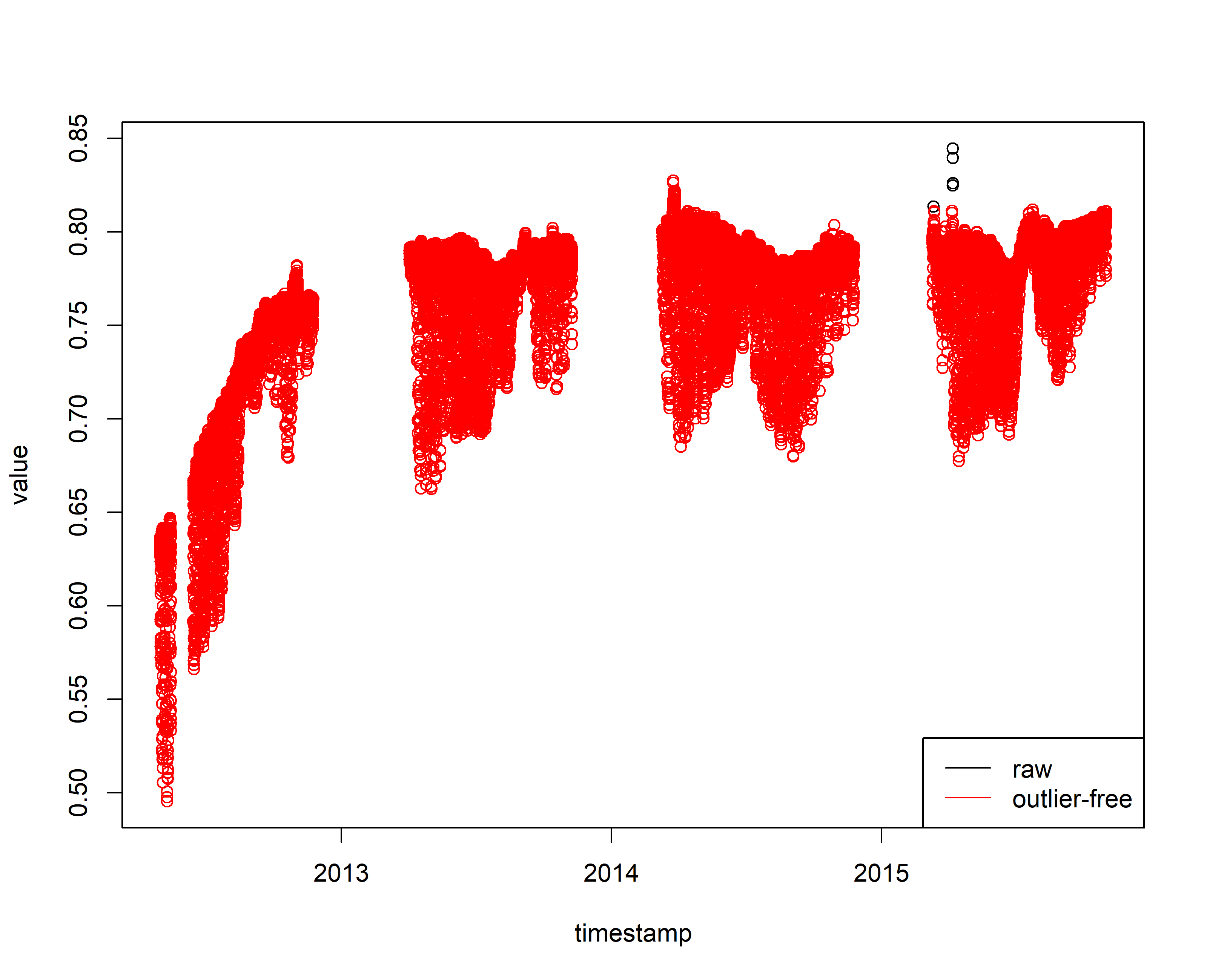
plot(sensor_raw_1h_df)
points(sensor_raw_1h_df_clean, col=2)
legend("bottomright", c("raw", "outlier-free"),
lty = 1, col = c("black", "red") )
# convert time stamp to character
sensor_raw_1h_df_clean$timestamp <- as.character(sensor_raw_1h_df_clean$timestamp)
4. Estimate zero-flow conditions (DTmax)
# see help page for a detailed description
#?tdm_dt.max
output.max <- tdm_dt.max(sensor_raw_1h_df_clean,
methods = c("pd","mw","dr","ed"),
det.pd = TRUE,
interpolate = FALSE,
max.days = 10,
ed.window = 2*60,
vpd.input = vpd_1h,
sr.input = rad_1h,
criteria = c(sr = 30, vpd = 0.1, cv = 0.5),
df = FALSE)
str(output.max)
## List of 17
## $ max.pd :'zoo' series from 2012-05-01 to 2015-10-31 23:00:00
## Data: num [1:30696] 0.637 0.637 0.637 0.637 0.637 ...
## Index: POSIXct[1:30696], format: "2012-05-01 00:00:00" "2012-05-01 01:00:00" ...
## $ max.mw :'zoo' series from 2012-05-01 to 2015-10-31 23:00:00
## Data: num [1:30696] 0.641 0.641 0.641 0.641 0.641 ...
## Index: POSIXct[1:30696], format: "2012-05-01 00:00:00" "2012-05-01 01:00:00" ...
## $ max.dr :'zoo' series from 2012-05-01 to 2015-10-31 23:00:00
## Data: num [1:30696] 0.641 0.641 0.641 0.641 0.641 ...
## Index: POSIXct[1:30696], format: "2012-05-01 00:00:00" "2012-05-01 01:00:00" ...
## $ max.ed :'zoo' series from 2012-04-30 12:00:00 to 2015-10-31 23:00:00
## Data: num [1:30697] 0.637 0.637 0.637 0.637 0.637 ...
## Index: POSIXct[1:30697], format: "2012-04-30 12:00:00" "2012-05-01 00:00:00" ...
## $ daily_max.pd:'zoo' series from 2012-05-01 to 2015-11-01
## Data: num [1:1280] 0.637 0.633 0.64 0.641 0.637 ...
## Index: Date[1:1280], format: "2012-05-01" "2012-05-02" ...
## $ daily_max.mw:'zoo' series from 2012-05-01 to 2015-11-01
## Data: num [1:1280] 0.641 0.641 0.641 0.641 0.641 ...
## Index: Date[1:1280], format: "2012-05-01" "2012-05-02" ...
## $ daily_max.dr:'zoo' series from 2012-05-01 to 2015-11-01
## Data: num [1:1280] 0.641 0.641 0.641 0.641 0.641 ...
## Index: Date[1:1280], format: "2012-05-01" "2012-05-02" ...
## $ daily_max.ed:'zoo' series from 2012-05-01 to 2015-11-01
## Data: num [1:1280] 0.637 0.633 0.64 0.639 0.637 ...
## Index: Date[1:1280], format: "2012-05-01" "2012-05-02" ...
## $ all.pd :'zoo' series from 2012-05-01 to 2015-10-31 23:00:00
## Data: num [1:30696] NA NA NA 0.637 NA ...
## Index: POSIXct[1:30696], format: "2012-05-01 00:00:00" "2012-05-01 01:00:00" ...
## $ all.ed :'zoo' series from 2012-05-01 to 2015-10-31 23:00:00
## Data: num [1:30696] NA NA NA 0.637 NA ...
## Index: POSIXct[1:30696], format: "2012-05-01 00:00:00" "2012-05-01 01:00:00" ...
## $ input :'zoo' series from 2012-05-01 to 2015-10-31 23:00:00
## Data: num [1:30696] 0.63 0.634 0.636 0.637 0.635 ...
## Index: POSIXct[1:30696], format: "2012-05-01 00:00:00" "2012-05-01 01:00:00" ...
## $ ed.criteria : Named num [1:3] 30 0.1 0.5
## ..- attr(*, "names")= chr [1:3] "sr" "vpd" "cv"
## $ methods : chr [1:4] "pd" "mw" "dr" "ed"
## $ k.pd :'zoo' series from 2012-05-01 to 2015-10-31 23:00:00
## Data: num [1:30696] 0.01012 0.00431 0.00118 0 0.00202 ...
## Index: POSIXct[1:30696], format: "2012-05-01 00:00:00" "2012-05-01 01:00:00" ...
## $ k.mw :'zoo' series from 2012-05-01 to 2015-10-31 23:00:00
## Data: num [1:30696] 0.01784 0.01199 0.00883 0.00764 0.00968 ...
## Index: POSIXct[1:30696], format: "2012-05-01 00:00:00" "2012-05-01 01:00:00" ...
## $ k.dr :'zoo' series from 2012-05-01 to 2015-10-31 23:00:00
## Data: num [1:30696] 0.017 0.01115 0.008 0.00681 0.00885 ...
## Index: POSIXct[1:30696], format: "2012-05-01 00:00:00" "2012-05-01 01:00:00" ...
## $ k.ed :'zoo' series from 2012-05-01 to 2015-10-31 23:00:00
## Data: num [1:30696] 0.01012 0.00431 0.00118 0 0.00202 ...
## Index: POSIXct[1:30696], format: "2012-05-01 00:00:00" "2012-05-01 01:00:00" ...
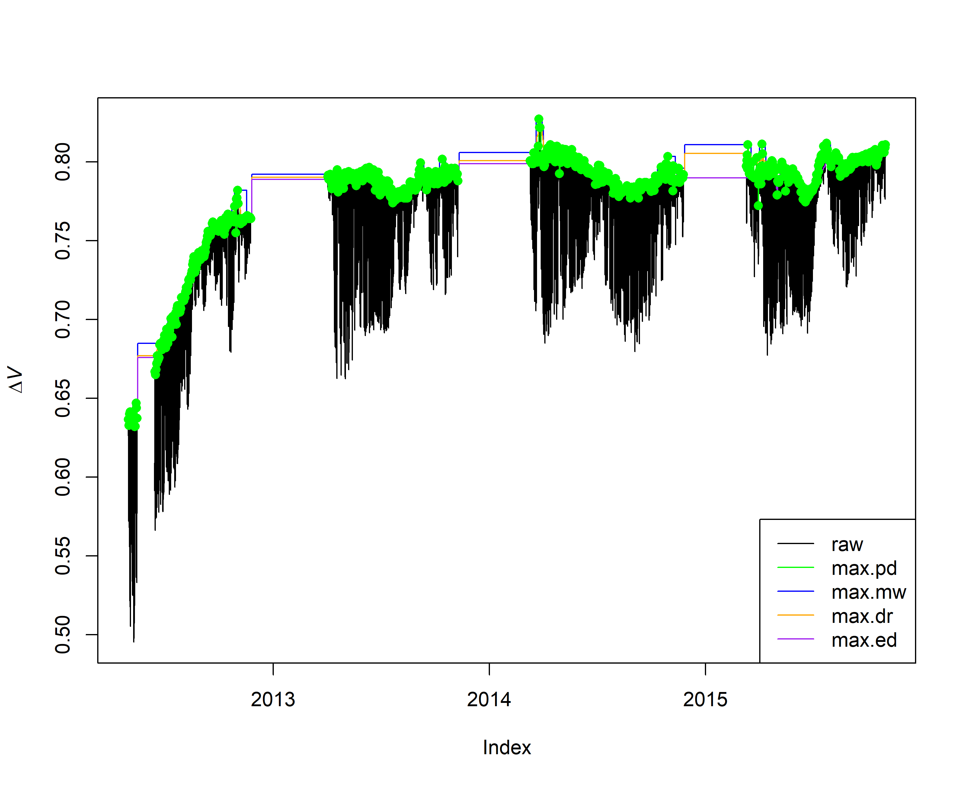
plot(output.max$input, ylab = expression(Delta*italic("V")))
lines(output.max$max.pd, col = "green")
lines(output.max$max.mw, col = "blue")
lines(output.max$max.dr, col = "orange")
lines(output.max$max.ed, col = "purple")
points(output.max$all.pd, col = "green", pch = 16)
legend("bottomright", c("raw", "max.pd", "max.mw", "max.dr", "max.ed"),
lty = 1, col = c("black", "green", "blue", "orange", "purple") )
# for visualizing, clip a single month (April, 2014)
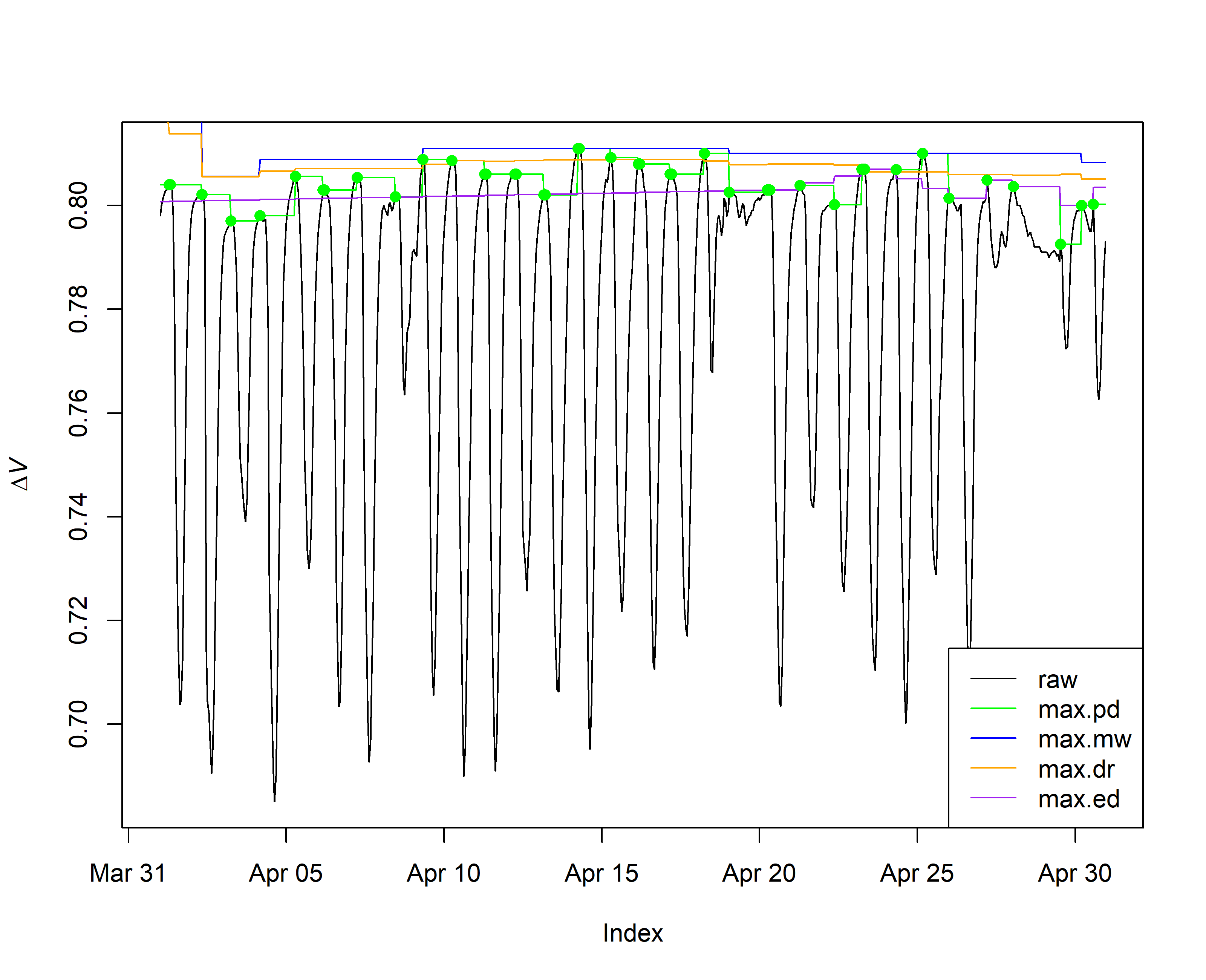
plot(window(output.max$input, start="2014-04-01 00:00:00", end="2014-04-30 23:30:00"), ylab = expression(Delta*italic("V")))
lines(window(output.max$max.pd, start="2014-04-01 00:00:00", end="2014-04-30 23:30:00"), col = "green")
lines(window(output.max$max.mw, start="2014-04-01 00:00:00", end="2014-04-30 23:30:00"), col = "blue")
lines(window(output.max$max.dr, start="2014-04-01 00:00:00", end="2014-04-30 23:30:00"), col = "orange")
lines(window(output.max$max.ed, start="2014-04-01 00:00:00", end="2014-04-30 23:30:00"), col = "purple")
points(window(output.max$all.pd, start="2014-04-01 00:00:00", end="2014-04-30 23:30:00"), col = "green", pch = 16)
legend("bottomright", c("raw", "max.pd", "max.mw", "max.dr", "max.ed"),
lty = 1, col = c("black", "green", "blue", "orange", "purple") )
5. Correction of sensor artifacts
Apply heartwood correction (if needed)
# The sapwood depth of the selected tree is 2.5 cm, and the probe length 2 cm, so no heartwood correction needs to be applied

# see help page for a detailed description
#?tdm_hw.cor

#SFD_cor = tdm_hw.cor(output.max,probe.length=20,
#                     sapwood.thickness= 25,
#                     df=F)
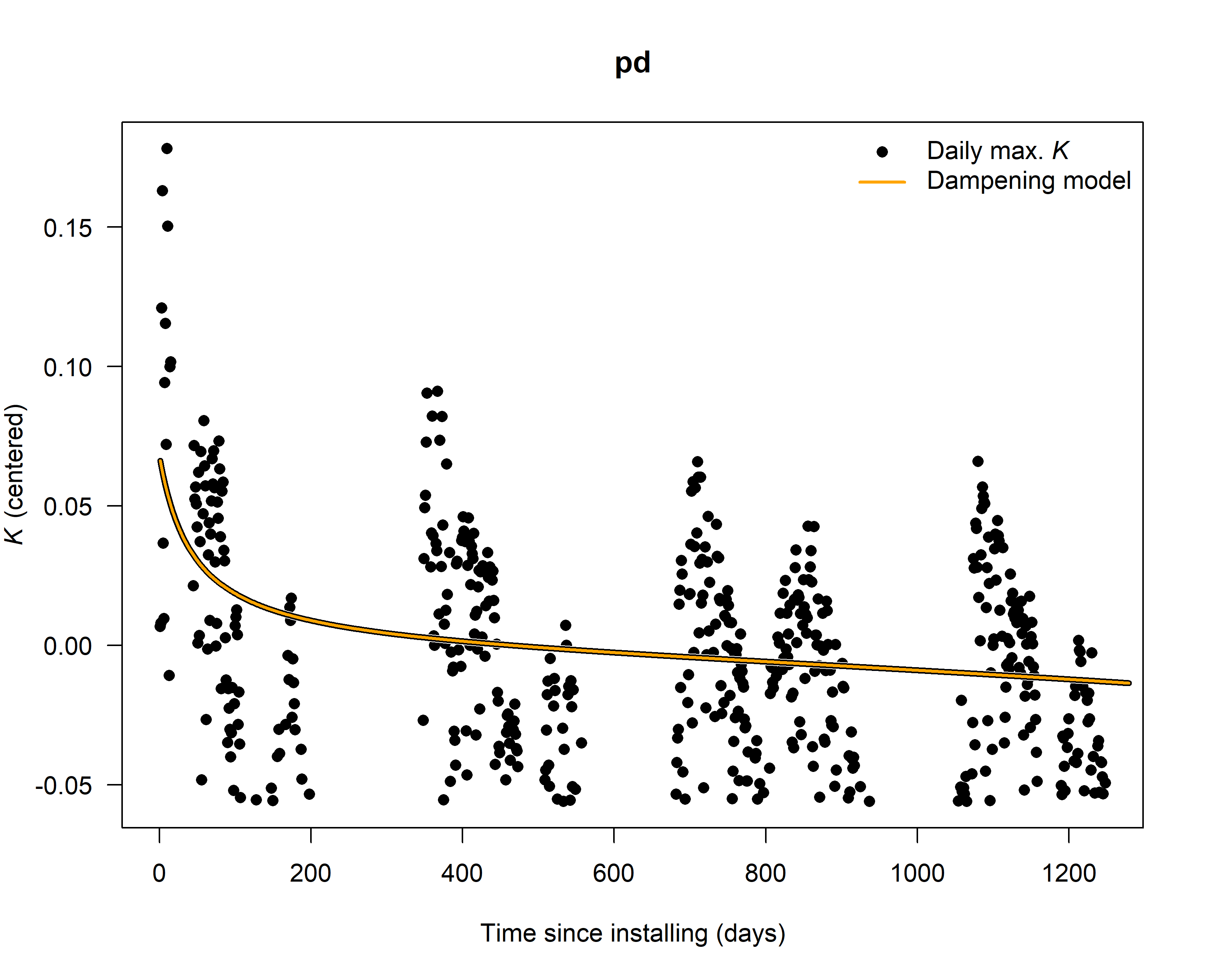
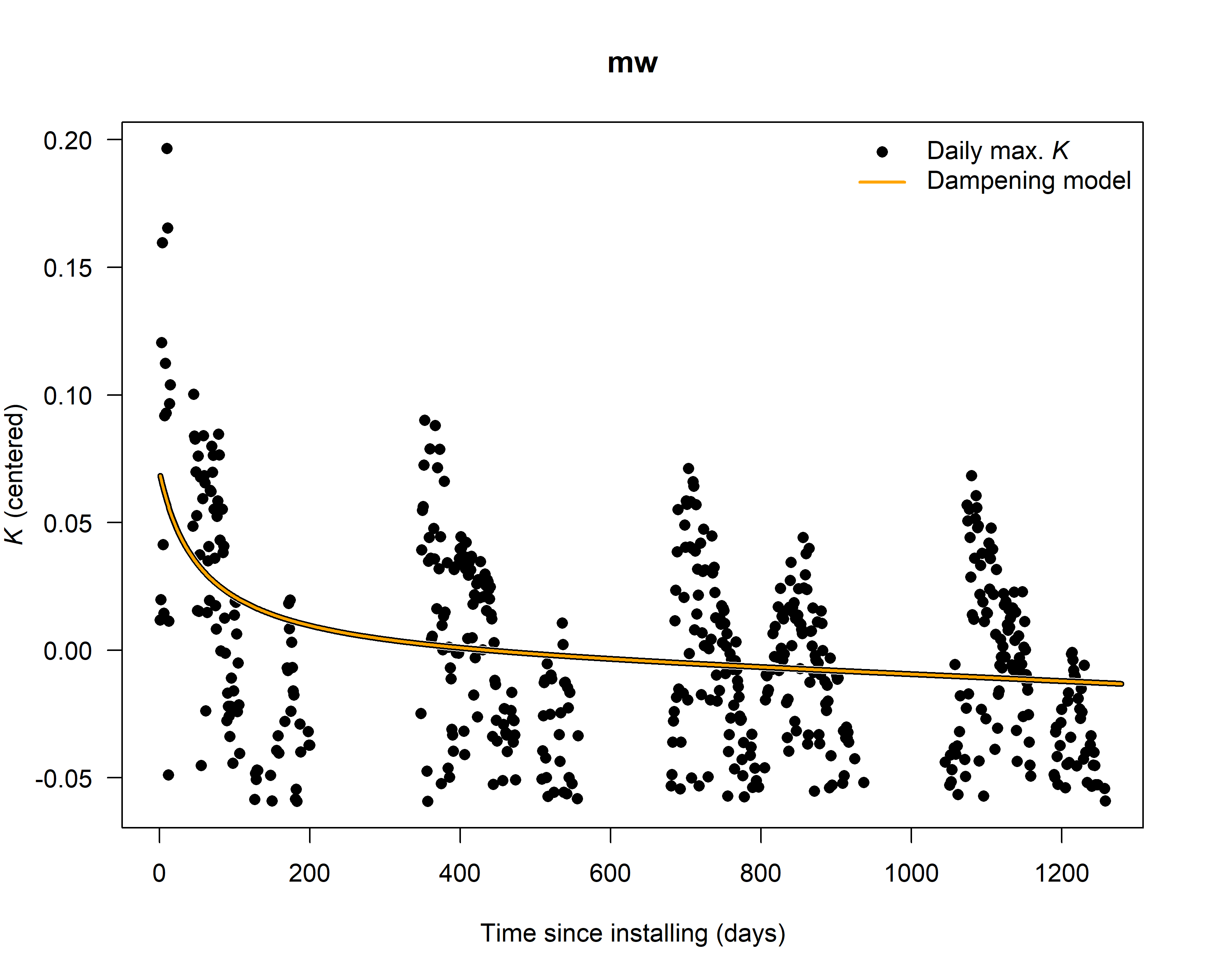
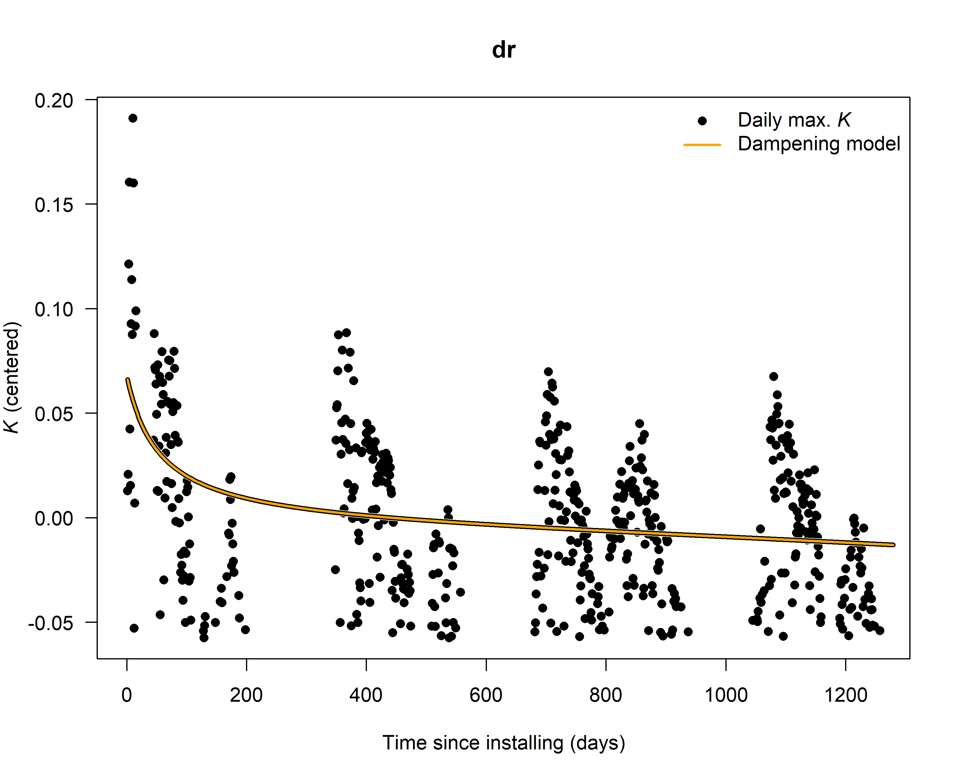
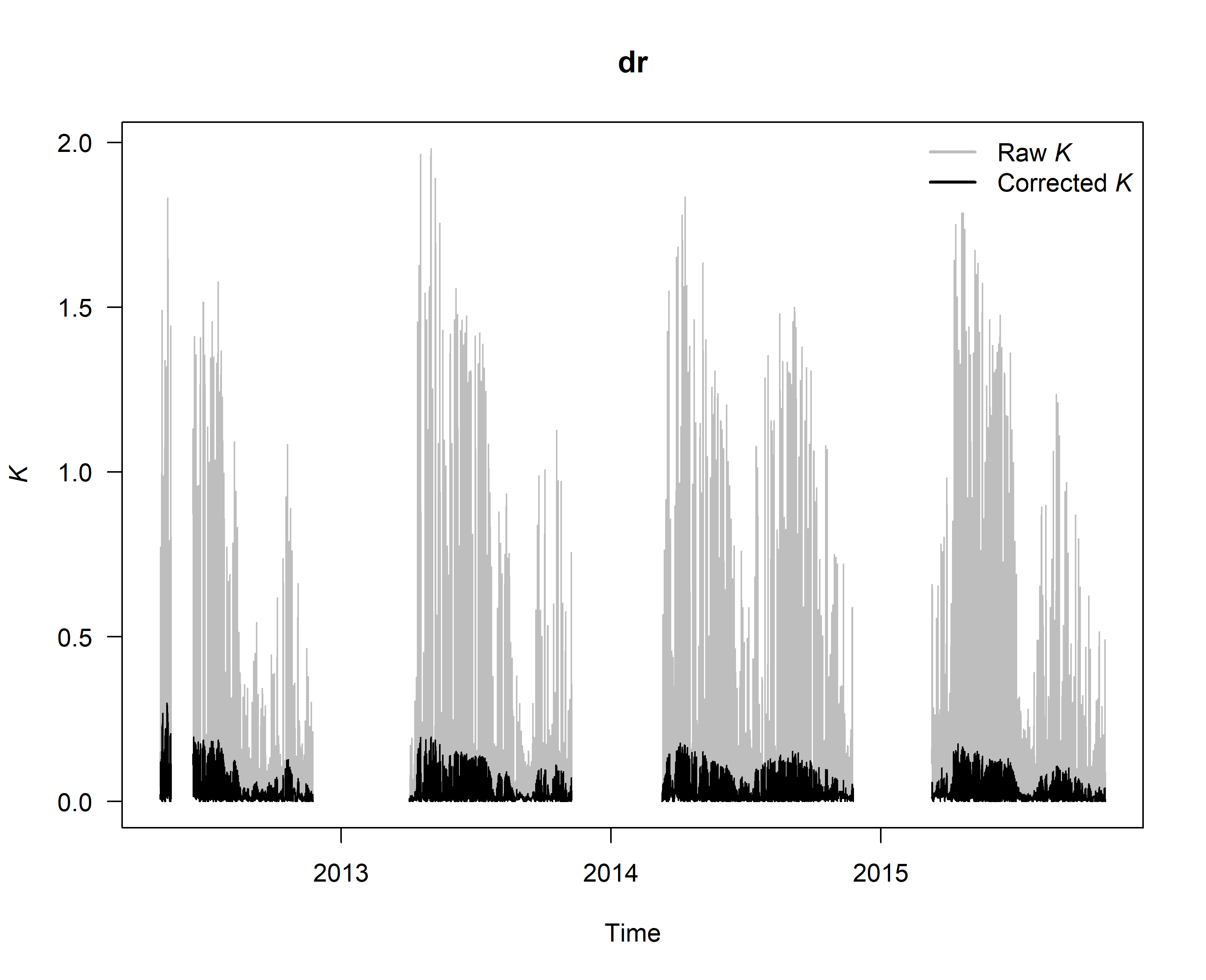
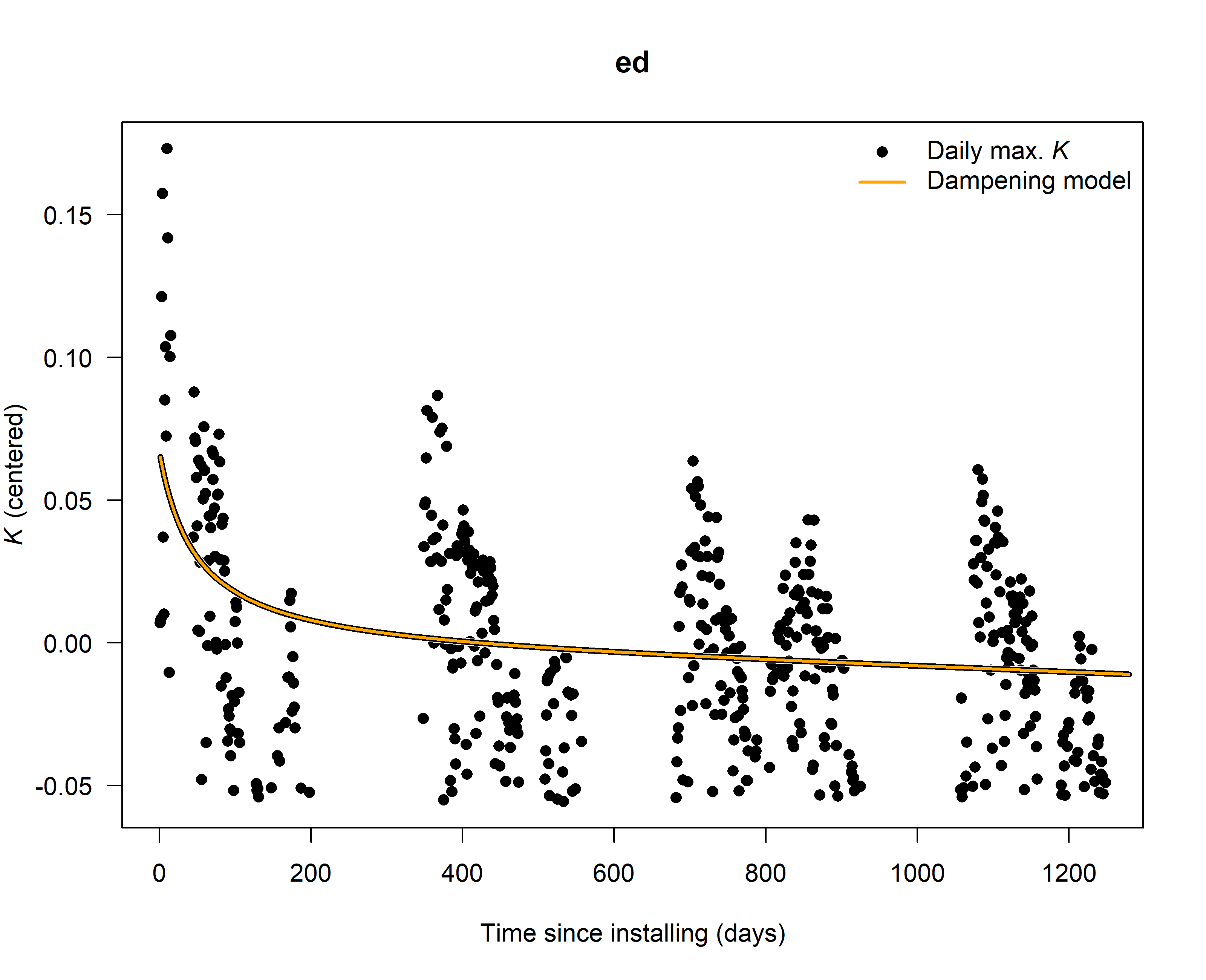
Check (and if existing) correct for dampening effects
# see help page for a detailed description
#?tdm_damp

SFD_damp <- tdm_damp(output.max,
                    k.threshold = 0.05,
                    make.plot = TRUE,
                    df = FALSE)


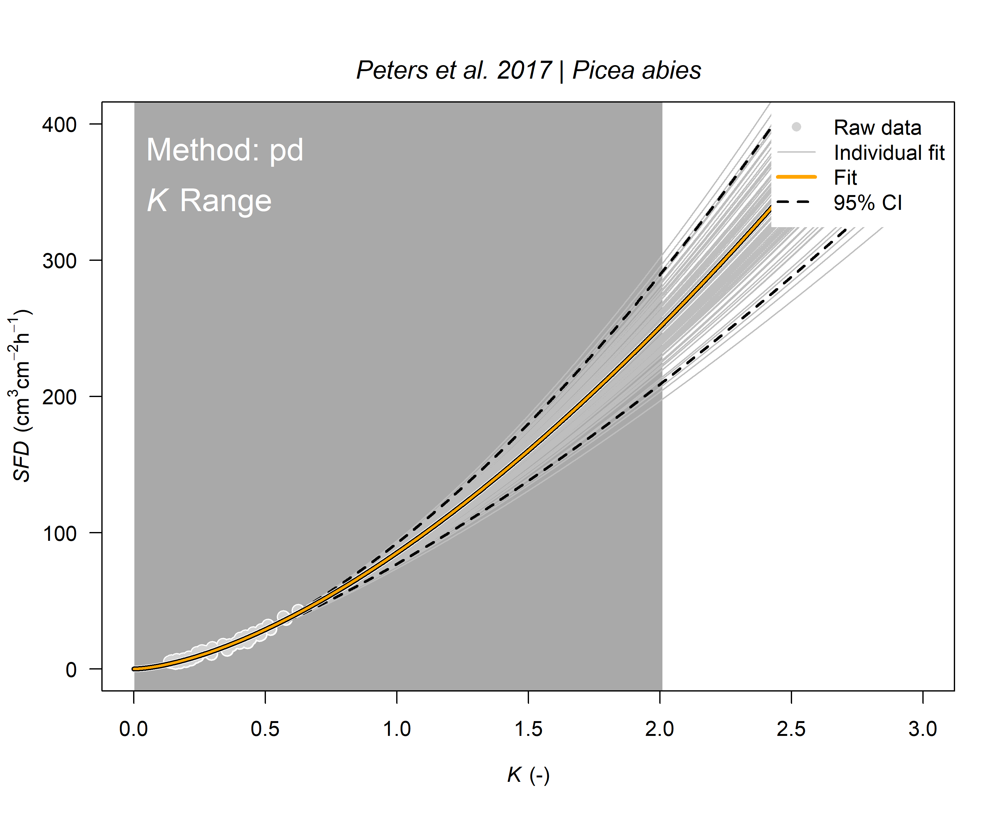
6. Calculate sap flux density
# see help page for a detailed description
#?tdm_cal.sfd

output.data <- tdm_cal.sfd(SFD_damp,
                          make.plot=T,
                          df=FALSE,
                          species="Picea abies")
str(output.data)
## List of 23
## $ max.pd :'zoo' series from 2012-05-01 to 2015-10-31 23:00:00
## Data: num [1:30696] 0.637 0.637 0.637 0.637 0.637 ...
## Index: POSIXct[1:30696], format: "2012-05-01 00:00:00" "2012-05-01 01:00:00" ...
## $ max.mw :'zoo' series from 2012-05-01 to 2015-10-31 23:00:00
## Data: num [1:30696] 0.641 0.641 0.641 0.641 0.641 ...
## Index: POSIXct[1:30696], format: "2012-05-01 00:00:00" "2012-05-01 01:00:00" ...
## $ max.dr :'zoo' series from 2012-05-01 to 2015-10-31 23:00:00
## Data: num [1:30696] 0.641 0.641 0.641 0.641 0.641 ...
## Index: POSIXct[1:30696], format: "2012-05-01 00:00:00" "2012-05-01 01:00:00" ...
## $ max.ed :'zoo' series from 2012-04-30 12:00:00 to 2015-10-31 23:00:00
## Data: num [1:30697] 0.637 0.637 0.637 0.637 0.637 ...
## Index: POSIXct[1:30697], format: "2012-04-30 12:00:00" "2012-05-01 00:00:00" ...
## $ daily_max.pd:'zoo' series from 2012-05-01 to 2015-11-01
## Data: num [1:1280] 0.637 0.633 0.64 0.641 0.637 ...
## Index: Date[1:1280], format: "2012-05-01" "2012-05-02" ...
## $ daily_max.mw:'zoo' series from 2012-05-01 to 2015-11-01
## Data: num [1:1280] 0.641 0.641 0.641 0.641 0.641 ...
## Index: Date[1:1280], format: "2012-05-01" "2012-05-02" ...
## $ daily_max.dr:'zoo' series from 2012-05-01 to 2015-11-01
## Data: num [1:1280] 0.641 0.641 0.641 0.641 0.641 ...
## Index: Date[1:1280], format: "2012-05-01" "2012-05-02" ...
## $ daily_max.ed:'zoo' series from 2012-05-01 to 2015-11-01
## Data: num [1:1280] 0.637 0.633 0.64 0.639 0.637 ...
## Index: Date[1:1280], format: "2012-05-01" "2012-05-02" ...
## $ all.pd :'zoo' series from 2012-05-01 to 2015-10-31 23:00:00
## Data: num [1:30696] NA NA NA 0.637 NA ...
## Index: POSIXct[1:30696], format: "2012-05-01 00:00:00" "2012-05-01 01:00:00" ...
## $ all.ed :'zoo' series from 2012-05-01 to 2015-10-31 23:00:00
## Data: num [1:30696] NA NA NA 0.637 NA ...
## Index: POSIXct[1:30696], format: "2012-05-01 00:00:00" "2012-05-01 01:00:00" ...
## $ input :'zoo' series from 2012-05-01 to 2015-10-31 23:00:00
## Data: num [1:30696] 0.63 0.634 0.636 0.637 0.635 ...
## Index: POSIXct[1:30696], format: "2012-05-01 00:00:00" "2012-05-01 01:00:00" ...
## $ ed.criteria : Named num [1:3] 30 0.1 0.5
## ..- attr(*, "names")= chr [1:3] "sr" "vpd" "cv"
## $ methods : chr [1:4] "pd" "mw" "dr" "ed"
## $ k.pd :'zoo' series from 2012-05-01 to 2015-10-31 23:00:00
## Data: num [1:30696] 0.06538 0.02787 0.00762 0 0.01306 ...
## Index: POSIXct[1:30696], format: "2012-05-01 00:00:00" "2012-05-01 01:00:00" ...
## $ k.mw :'zoo' series from 2012-05-01 to 2015-10-31 23:00:00
## Data: num [1:30696] 0.1102 0.074 0.0545 0.0472 0.0598 ...
## Index: POSIXct[1:30696], format: "2012-05-01 00:00:00" "2012-05-01 01:00:00" ...
## $ k.dr :'zoo' series from 2012-05-01 to 2015-10-31 23:00:00
## Data: num [1:30696] 0.1091 0.0716 0.0514 0.0437 0.0568 ...
## Index: POSIXct[1:30696], format: "2012-05-01 00:00:00" "2012-05-01 01:00:00" ...
## $ k.ed :'zoo' series from 2012-05-01 to 2015-10-31 23:00:00
## Data: num [1:30696] 0.06629 0.02826 0.00773 0 0.01324 ...
## Index: POSIXct[1:30696], format: "2012-05-01 00:00:00" "2012-05-01 01:00:00" ...
## $ sfd.pd :'zoo' series from 2012-05-01 to 2015-10-31 23:00:00
## Data: num [1:30696, 1:4] 0.06538 0.02787 0.00762 0 0.01305 ...
## ..- attr(*, "dimnames")=List of 2
## .. ..$ : chr [1:30696] "65405" "27880" "7625" "1" ...
## .. ..$ : chr [1:4] "k" "sfd" "q025" "q975"
## Index: POSIXct[1:30696], format: "2012-05-01 00:00:00" "2012-05-01 01:00:00" ...
## $ sfd.mw :'zoo' series from 2012-05-01 to 2015-10-31 23:00:00
## Data: num [1:30696, 1:4] 0.1102 0.074 0.0545 0.0472 0.0598 ...
## ..- attr(*, "dimnames")=List of 2
## .. ..$ : chr [1:30696] "110202" "74074" "54571" "47227" ...
## .. ..$ : chr [1:4] "k" "sfd" "q025" "q975"
## Index: POSIXct[1:30696], format: "2012-05-01 00:00:00" "2012-05-01 01:00:00" ...
## $ sfd.dr :'zoo' series from 2012-05-01 to 2015-10-31 23:00:00
## Data: num [1:30696, 1:4] 0.1091 0.0716 0.0514 0.0437 0.0568 ...
## ..- attr(*, "dimnames")=List of 2
## .. ..$ : chr [1:30696] "109147" "71628" "51375" "43749" ...
## .. ..$ : chr [1:4] "k" "sfd" "q025" "q975"
## Index: POSIXct[1:30696], format: "2012-05-01 00:00:00" "2012-05-01 01:00:00" ...
## $ sfd.ed :'zoo' series from 2012-05-01 to 2015-10-31 23:00:00
## Data: num [1:30696, 1:4] 0.06629 0.02826 0.00773 0 0.01324 ...
## ..- attr(*, "dimnames")=List of 2
## .. ..$ : chr [1:30696] "66312" "28267" "7731" "1" ...
## .. ..$ : chr [1:4] "k" "sfd" "q025" "q975"
## Index: POSIXct[1:30696], format: "2012-05-01 00:00:00" "2012-05-01 01:00:00" ...
## $ model.ens :'data.frame': 3001242 obs. of 4 variables:
## ..$ k : num [1:3001242] 0e+00 1e-06 2e-06 3e-06 4e-06 5e-06 6e-06 7e-06 8e-06 9e-06 ...
## ..$ sfd : num [1:3001242] 0.00 1.82e-06 3.64e-06 5.45e-06 7.27e-06 ...
## ..$ q025: num [1:3001242] 0.00 9.71e-07 1.94e-06 2.91e-06 3.88e-06 ...
## ..$ q975: num [1:3001242] 0.00 3.75e-06 7.51e-06 1.13e-05 1.50e-05 ...
## $ out.param :'data.frame': 1 obs. of 7 variables:
## ..$ n : int 100
## ..$ a_mu : num 84.8
## ..$ a_sd : num 4.19
## ..$ log.a_mu: num 4.44
## ..$ log.a_sd: num 0.05
## ..$ b_mu : num 1.55
## ..$ b_sd : num 0.0586
output.data$out.param
## n a_mu a_sd log.a_mu log.a_sd b_mu b_sd
## 1 100 84.82307 4.190217 4.43934 0.050006 1.551006 0.05861681
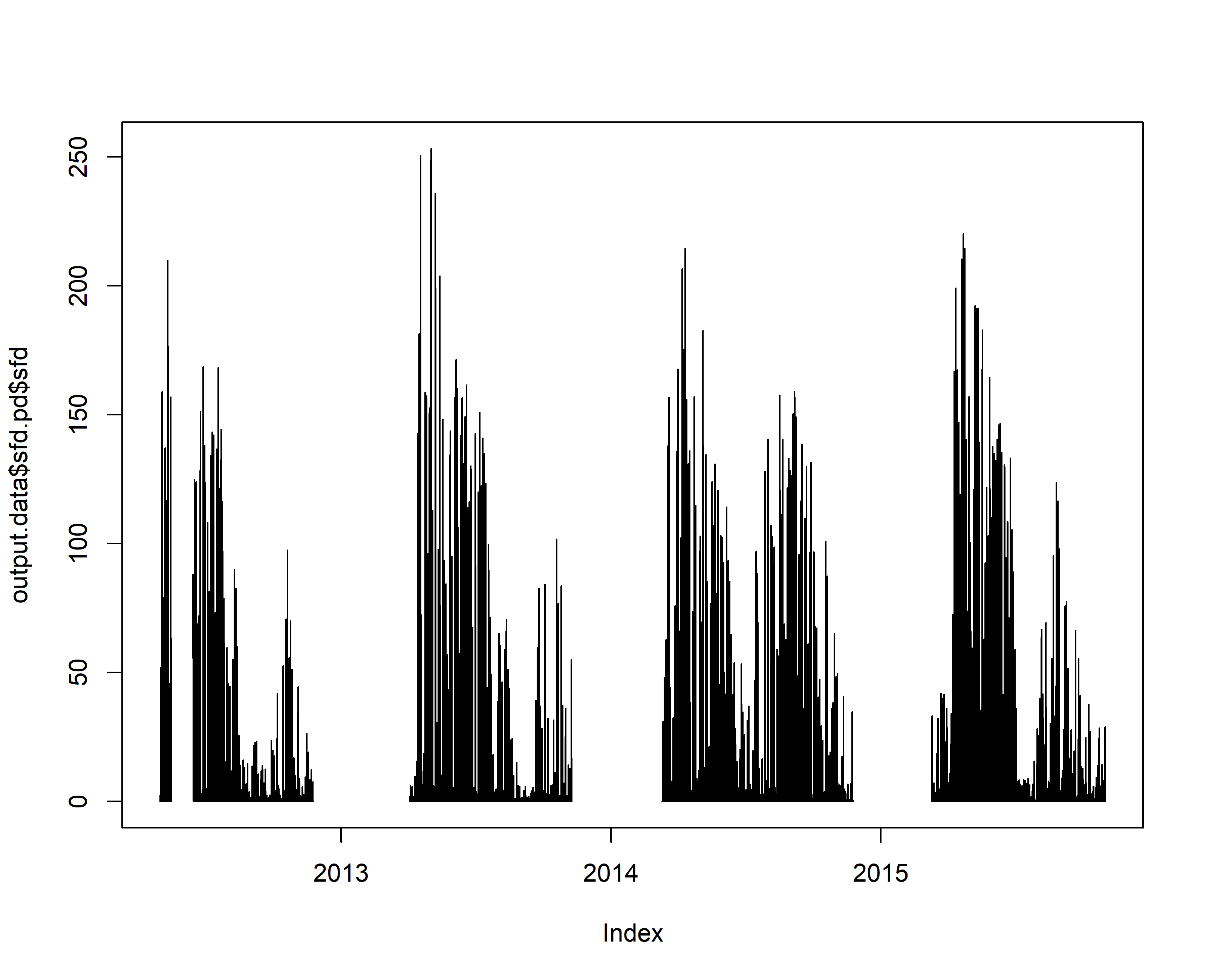
plot(output.data$sfd.pd$sfd)
7. Calculate crown conductance to water, and its response to VPD
# see help page for a detailed description
#?out.data

output <- out.data(input=output.data$sfd.pd$sfd,
                  vpd.input=vpd_1h,
                  sr.input=rad_1h,
                  prec.input=prc_1day,
                  low.sr = 150, peak.sr=300, vpd.cutoff= 0.5, prec.lim=1,
                  method="env.filt", max.quant=0.99, make.plot=TRUE)
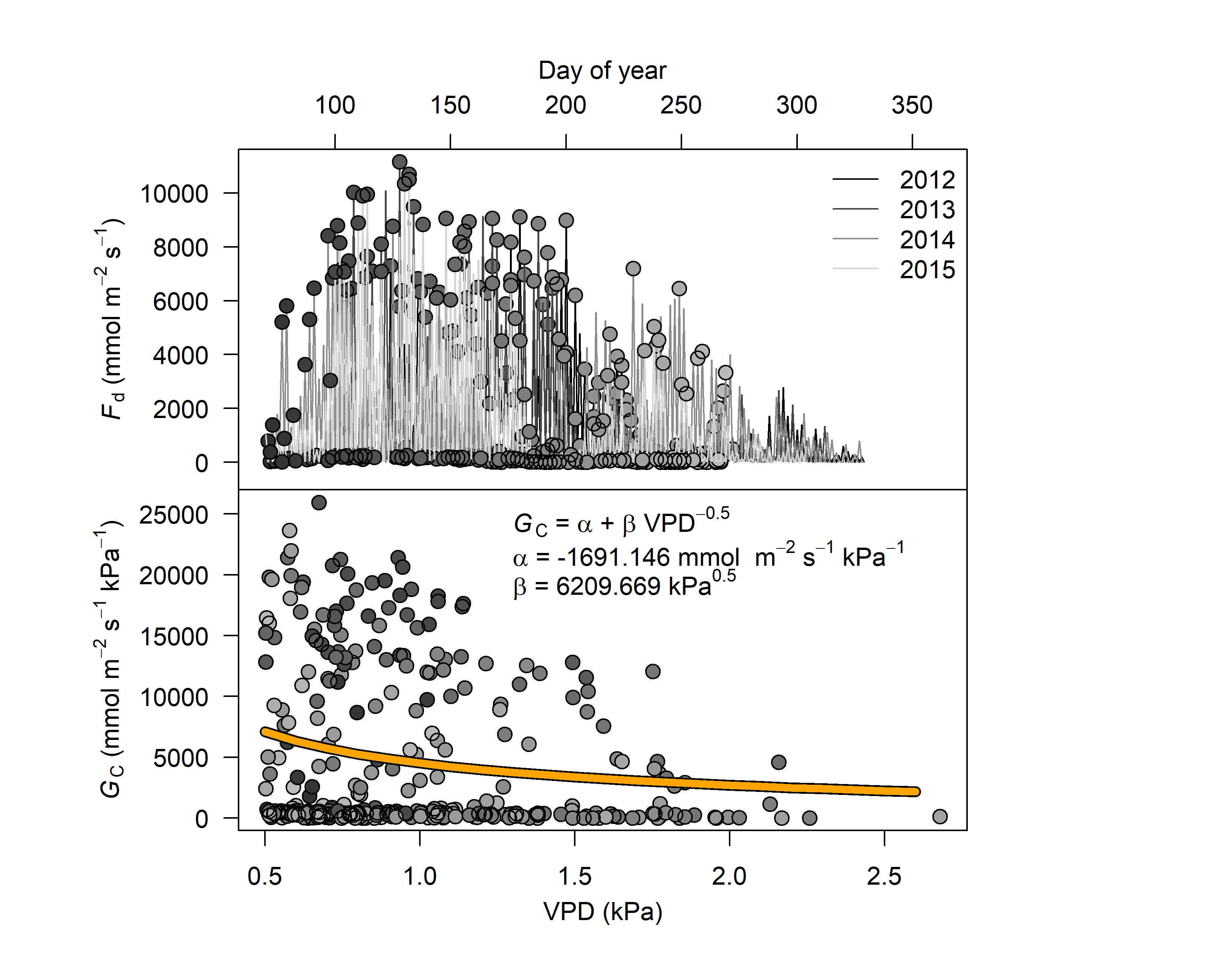
str(output)
## List of 4
##  $ raw         :'data.frame':	30696 obs. of  12 variables:
##   ..$ timestamp: POSIXct[1:30696], format: "2012-05-01 00:00:00" "2012-05-01 01:00:00" ...
##   ..$ year     : num [1:30696] 2012 2012 2012 2012 2012 ...
##   ..$ doy      : num [1:30696] 122 122 122 122 122 122 122 122 122 122 ...
##   ..$ hour     : num [1:30696] 0 1 2 3 4 5 6 7 8 9 ...
##   ..$ sr       : num [1:30696] 0.6 0.6 0.6 0.6 0.6 ...
##   ..$ sr.day   : num [1:30696] 183 183 183 183 183 ...
##   ..$ vpd      : num [1:30696] 0.0595 0.047 0.0415 0.0434 0.0392 ...
##   ..$ vpd.filt : num [1:30696] NA NA NA NA NA NA NA NA NA NA ...
##   ..$ prec.day : num [1:30696] 11.1 11.1 11.1 11.1 11.1 ...
##   ..$ fd       : num [1:30696] 188.1 49.87 6.64 0 15.31 ...
##   ..$ gc       : num [1:30696] 3159 1061 160 0 391 ...
##   ..$ gc.filt  : num [1:30696] NA NA NA NA NA NA NA NA NA NA ...
##  $ peak.mean   :'data.frame':	1279 obs. of  4 variables:
##   ..$ timestamp: chr [1:1279] "2012-05-01" "2012-05-02" "2012-05-03" "2012-05-04" ...
##   ..$ vpd.filt : num [1:1279] NA NA 0.622 0.855 NA ...
##   ..$ gc.filt  : num [1:1279] NA NA 19394 851 NA ...
##   ..$ gc.norm  : num [1:1279] NA NA 0.9056 0.0397 NA ...
##  $ sum.mod     :List of 11
##   ..$ formula     :Class 'formula'  language y ~ a + d * x^(-0.5)
##   .. .. ..- attr(*, ".Environment")=<environment: 0x000000004fdd1e60>
##   ..$ residuals   : num [1:329] 13212 -4175 5768 -3197 8253 ...
##   ..$ sigma       : num 6556
##   ..$ df          : int [1:2] 2 327
##   ..$ cov.unscaled: num [1:2, 1:2] 0.0961 -0.0874 -0.0874 0.082
##   .. ..- attr(*, "dimnames")=List of 2
##   .. .. ..$ : chr [1:2] "a" "d"
##   .. .. ..$ : chr [1:2] "a" "d"
##   ..$ call        : language stats::nls(formula = y ~ a + d * x^(-0.5), data = df, start = list(a = 1,      d = 1), algorithm = "default", con| __truncated__ ...
##   ..$ convInfo    :List of 5
##   .. ..$ isConv     : logi TRUE
##   .. ..$ finIter    : int 1
##   .. ..$ finTol     : num 4.93e-09
##   .. ..$ stopCode   : int 0
##   .. ..$ stopMessage: chr "converged"
##   ..$ control     :List of 5
##   .. ..$ maxiter  : num 50
##   .. ..$ tol      : num 1e-05
##   .. ..$ minFactor: num 0.000977
##   .. ..$ printEval: logi FALSE
##   .. ..$ warnOnly : logi FALSE
##   ..$ na.action   : NULL
##   ..$ coefficients: num [1:2, 1:4] -1691.146 6209.669 2032.428 1877.487 -0.832 ...
##   .. ..- attr(*, "dimnames")=List of 2
##   .. .. ..$ : chr [1:2] "a" "d"
##   .. .. ..$ : chr [1:4] "Estimate" "Std. Error" "t value" "Pr(>|t|)"
##   ..$ parameters  : num [1:2, 1:4] -1691.146 6209.669 2032.428 1877.487 -0.832 ...
##   .. ..- attr(*, "dimnames")=List of 2
##   .. .. ..$ : chr [1:2] "a" "d"
##   .. .. ..$ : chr [1:4] "Estimate" "Std. Error" "t value" "Pr(>|t|)"
##   ..- attr(*, "class")= chr "summary.nls"
##  $ sum.mod.norm:List of 11
##   ..$ formula     :Class 'formula'  language y ~ a + d * x^(-0.5)
##   .. .. ..- attr(*, ".Environment")=<environment: 0x000000004fdd1e60>
##   ..$ residuals   : num [1:329] 0.617 -0.195 0.269 -0.149 0.385 ...
##   ..$ sigma       : num 0.306
##   ..$ df          : int [1:2] 2 327
##   ..$ cov.unscaled: num [1:2, 1:2] 0.0961 -0.0874 -0.0874 0.082
##   .. ..- attr(*, "dimnames")=List of 2
##   .. .. ..$ : chr [1:2] "a" "d"
##   .. .. ..$ : chr [1:2] "a" "d"
##   ..$ call        : language stats::nls(formula = y ~ a + d * x^(-0.5), data = df_n, start = list(a = 1,      d = 1), algorithm = "default", c| __truncated__ ...
##   ..$ convInfo    :List of 5
##   .. ..$ isConv     : logi TRUE
##   .. ..$ finIter    : int 1
##   .. ..$ finTol     : num 2.55e-09
##   .. ..$ stopCode   : int 0
##   .. ..$ stopMessage: chr "converged"
##   ..$ control     :List of 5
##   .. ..$ maxiter  : num 50
##   .. ..$ tol      : num 1e-05
##   .. ..$ minFactor: num 0.000977
##   .. ..$ printEval: logi FALSE
##   .. ..$ warnOnly : logi FALSE
##   ..$ na.action   : NULL
##   ..$ coefficients: num [1:2, 1:4] -0.079 0.29 0.0949 0.0877 -0.8321 ...
##   .. ..- attr(*, "dimnames")=List of 2
##   .. .. ..$ : chr [1:2] "a" "d"
##   .. .. ..$ : chr [1:4] "Estimate" "Std. Error" "t value" "Pr(>|t|)"
##   ..$ parameters  : num [1:2, 1:4] -0.079 0.29 0.0949 0.0877 -0.8321 ...
##   .. ..- attr(*, "dimnames")=List of 2
##   .. .. ..$ : chr [1:2] "a" "d"
##   .. .. ..$ : chr [1:4] "Estimate" "Std. Error" "t value" "Pr(>|t|)"
##   ..- attr(*, "class")= chr "summary.nls"
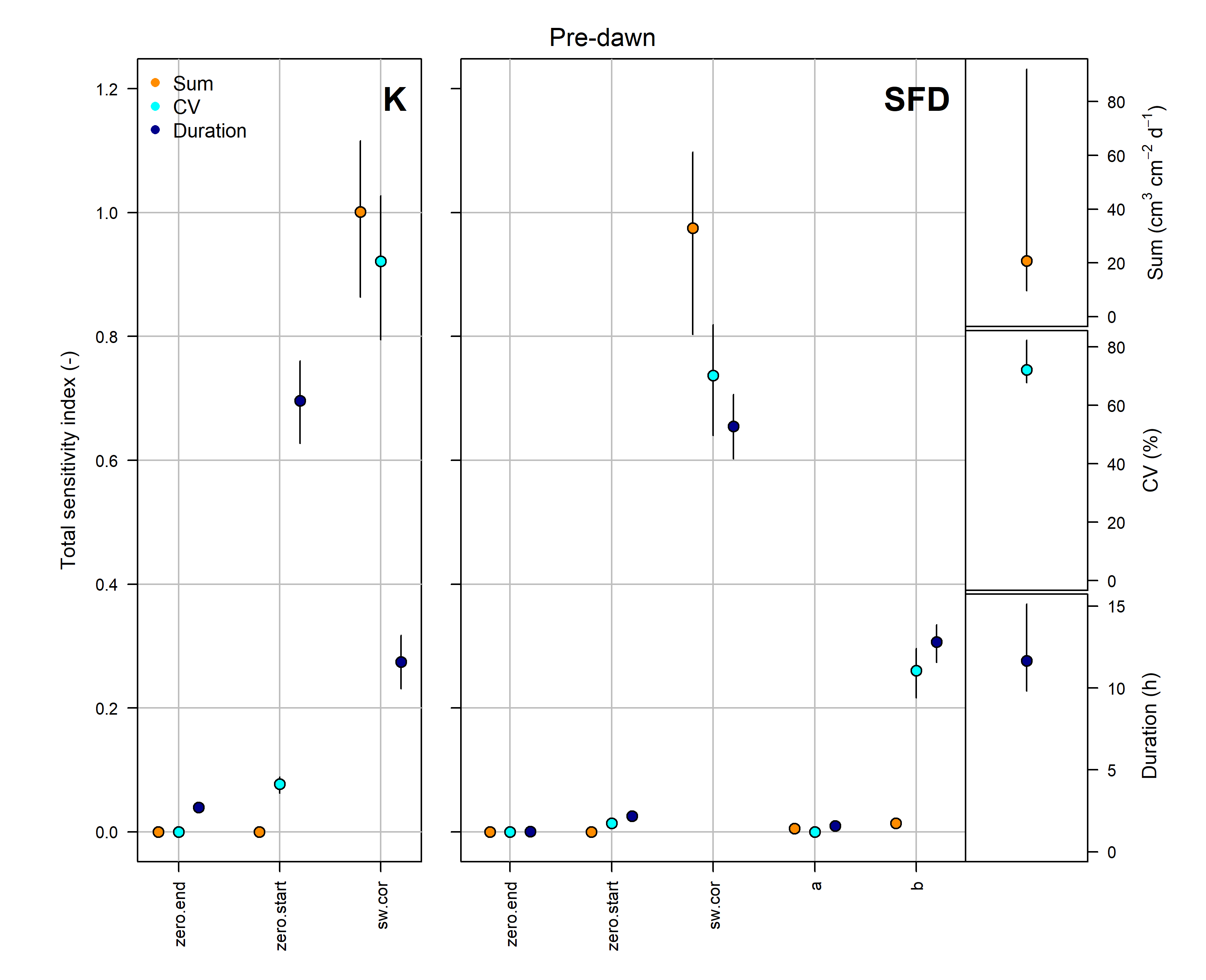
8. Estimate uncertainties with a thorough global sensitivity/uncertainty analysis
# The implemented methods for the global sensitivity and uncertainty analysis are computational demanding. Here, for illustration purposes we have selected a sub-period of few months.

# see help page for a detailed description
#?tdm_uncertain
output <- tdm_uncertain(window(sensor_raw_1h,
                              start = "2014-03-01 00:00:00",
                              end = "2014-09-01 00:00:00"),
                       probe.length=20,
                       method="pd",
                       n=2000,
                       sw.cor=25,
                       sw.sd=16,
                       log.a_mu=output.data$out.param$log.a_mu,
                       log.a_sd=output.data$out.param$log.a_sd,
                       b_mu=output.data$out.param$b_mu,
                       b_sd=output.data$out.param$b_sd,
                       make.plot=TRUE)
9. Using TREX
For use in publication, the reference is:
citation("TREX")
##
## To cite package 'TREX' in publications use:
##
##   Richard Peters, Christoforos Pappas and Alexander Hurley (2020).
##   TREX: TRree sap flow EXtractor. R package version 0.0.0.9000.
##   https://the-hull.github.io/TREX/
##
## A BibTeX entry for LaTeX users is
##
##   @Manual{,
##     title = {TREX: TRree sap flow EXtractor},
##     author = {Richard Peters and Christoforos Pappas and Alexander Hurley},
##     year = {2020},
##     note = {R package version 0.0.0.9000},
##     url = {https://the-hull.github.io/TREX/},
##   }
10. References
- Richard Peters, Christoforos Pappas and Alexander Hurley (2020). TREX: TRree sap flow EXtractor. R package version 0.0.0.9000. https://the-hull.github.io/TREX/
11. Contact
For questions, please get in touch with Chris Pappas