Analysis Workflow

1. Background

The package treenetproc cleans, processes and visualises highly resolved time series of dendrometer data in two steps; raw dendrometer data is aligned to regular time intervals (level 1: L1) and cleaned (level 2: L2).

In an optional third step several commonly used characteristics such as the start and end of stem growth can be calculated.

This tutorial presents an example for processing a single dendrometer time-series, yet the package does allow for processing of multiple time-series in one run.

2. Set-up Steps

# install if necessary
packages <- (c("devtools","zoo","chron","dplyr","viridis", "RCurl", "DT"))
install.packages(setdiff(packages, rownames(installed.packages())))
devtools::install_github("treenet/treenetproc")

library(treenetproc)
library(zoo)
library(chron)
library(viridis)
library(dplyr)

# helper functions
left <-  function(string, char){substr(string, 1,char)}
right <-  function (string, char){substr(string,nchar(string)-(char-1),nchar(string))}

3. Import data (L0)

Raw dendrometer and temperature data can be provided as input. Providing temperature data is optional. However, temperature data increases the quality of error detection and processing.

The raw dendrometer or climate data can be provided in long format. Data of multiple sensors can either be specified in a column named series to separate the sensors.

Dendrometer data always has to be provided in microns. In addition, a column named ts with timestamps in any standard date format (default is date_format = "%Y-%m-%d %H:%M:%S") is required.

Dendrometer data:

# import table data
url_dendrodata <- RCurl::getURL("https://raw.githubusercontent.com/deep-org/workshop_data/master/esa-workshop2020/N13Ad_S1_radius%20(micron).txt")
dendro_data_L0<-read.table(text = url_dendrodata, 
                           header=T,
                           sep="\t")

# Illustrate the structure of the input data:
str(dendro_data_L0)
## 'data.frame':	26304 obs. of  3 variables:
##  $ series: Factor w/ 1 level "LOT_N13Ad_S1": 1 1 1 1 1 1 1 1 1 1 ...
##  $ ts    : Factor w/ 26304 levels "2008-01-01 00:00:00",..: 1 2 3 4 5 6 7 8 9 10 ...
##  $ value : num  415 422 418 414 417 414 411 414 412 408 ...

# Table structure:
head(dendro_data_L0)
##         series                  ts value
## 1 LOT_N13Ad_S1 2008-01-01 00:00:00   415
## 2 LOT_N13Ad_S1 2008-01-01 01:00:00   422
## 3 LOT_N13Ad_S1 2008-01-01 02:00:00   418
## 4 LOT_N13Ad_S1 2008-01-01 03:00:00   414
## 5 LOT_N13Ad_S1 2008-01-01 04:00:00   417
## 6 LOT_N13Ad_S1 2008-01-01 05:00:00   414

# grab years
years <-left(dendro_data_L0[,"ts"],4)

# plotting
par(mfrow=c(1,1))
par(mar = c(5, 5, 5, 5))
for(y in 1:length(unique(years))){
  # selected year
  sel<-dendro_data_L0[which(years==unique(years)[y]),]
  # handle first year
  if(y==1){
    plot(difftime(as.POSIXct(sel$ts,format="%Y-%m-%d %H:%M:%S",tz="GMT"),
                  as.POSIXct(paste0(unique(years)[y],"-01-01 00:00:00"),
                             format="%Y-%m-%d %H:%M:%S",tz="GMT"),
                  units = "days"),
         sel$value,
         ylab=expression("L0 ("*mu*"m)"),
         xlab="Day of year",type="l",
         col=viridis(length(unique(years)))[y],
         xlim=c(0,365),
         ylim=c(min(dendro_data_L0$value,na.rm=T),
                max(dendro_data_L0$value,na.rm=T)),
         main=unique(dendro_data_L0$series))
    
    legend("bottomright",
           as.character(unique(years)[-4]),
           col=viridis(length(unique(years))),
           bty="n",lty=1)
    # add other years
  }else{
    lines(difftime(as.POSIXct(sel$ts,format="%Y-%m-%d %H:%M:%S",tz="GMT"),
                   as.POSIXct(paste0(unique(years)[y],"-01-01 00:00:00"),
                              format="%Y-%m-%d %H:%M:%S",tz="GMT"),
                   units = "days"),
          sel$value,
          col=viridis(length(unique(years)))[y])}}

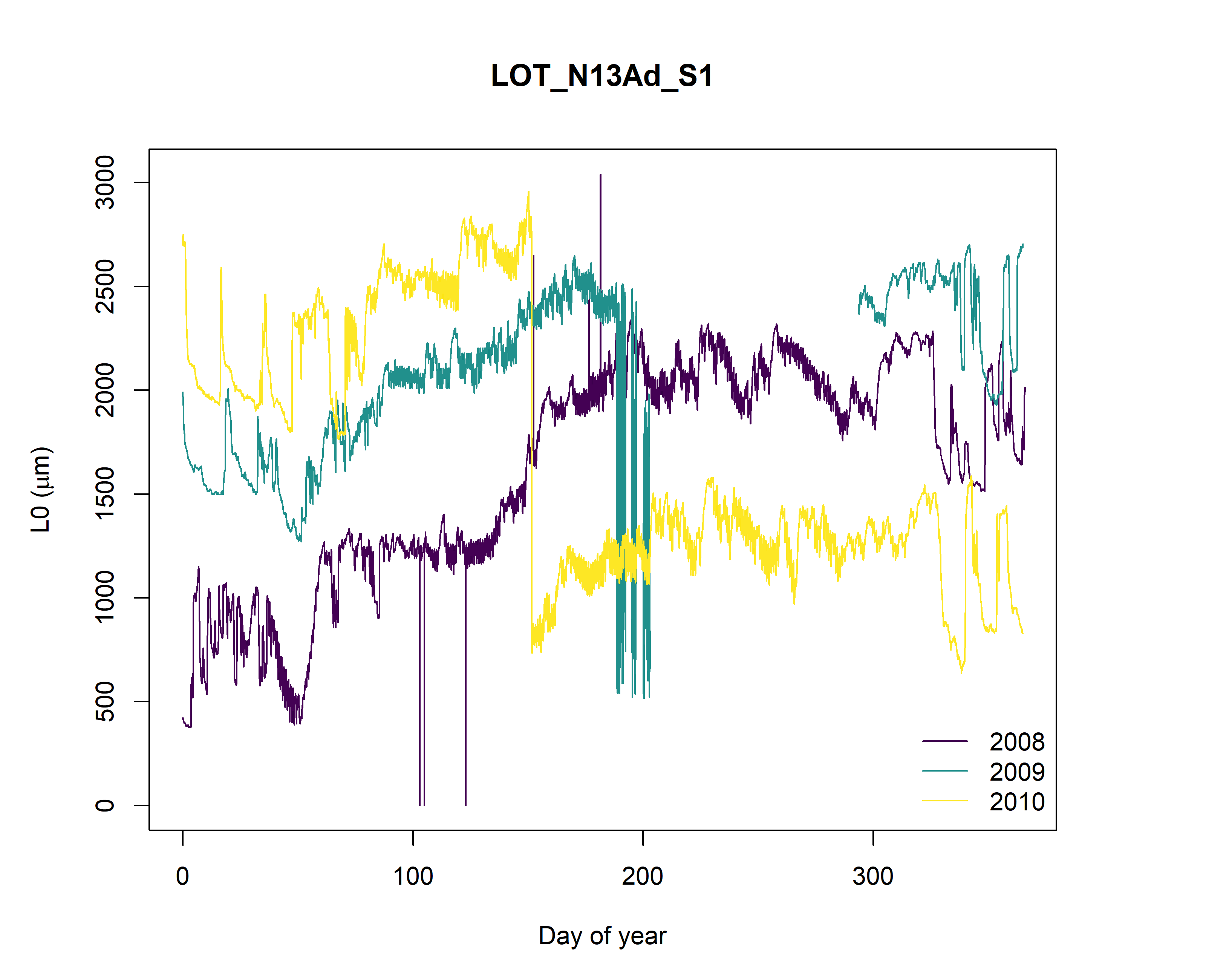
Figure: Here we plotted all three years of raw dendrometer data (L0; radial variability in micron collected from a Picea abies tree (S1) growing in the valley bottom (N13Ad) in the Lötschental (LOT; Switzerland). See Pappas et al. (2020; Ecography) for more site specific information.

Multiple data issues are present within the data, including; outliers in 2008, sensor failure in 2009 and a measurement jump due to reinstalling the sensor in 2010.

Temperature Data

If temperature data is provided along with dendrometer data, the name of the temperature data series has to contain the string temp to be identified as temperature data.

# import table data
url_tempdata <- RCurl::getURL("https://raw.githubusercontent.com/deep-org/workshop_data/master/esa-workshop2020/N13Ad_S1_Temperature%20(degree%20C).txt")
temp_data  <-read.table(text = url_tempdata,
                        header=T,sep="\t")

# Matching temperature with dendrometer data:
temp_data_L0<-temp_data[which(temp_data$ts%in%dendro_data_L0$ts), ]

# Plotting daily aggregated temperature:
d_temp_data<-aggregate(temp_data_L0$value,
                       by=list(as.Date(temp_data_L0$ts)),
                       mean,
                       na.rm=T)


years <-left(d_temp_data[,1],4)
par(mfrow=c(1,1))
par(mar = c(5, 5, 5, 5))

# loop through years
for(y in 1:length(unique(years))){
  
  sel<-d_temp_data[which(years==unique(years)[y]),]
  
  # handle first year
  if(y==1){
    plot(difftime(as.POSIXct(sel[,1],format="%Y-%m-%d",tz="GMT"),
                  as.POSIXct(paste0(unique(years)[y],"-01-01 00:00:00"),
                             format="%Y-%m-%d %H:%M:%S",tz="GMT"),
                  units = "days"),
         sel[,2],
         ylab=expression("Daily temperature ("*degree*"C)"),
         xlab="Day of year",
         type="p",
         pch=16,
         col=rainbow(length(unique(years)))[y],
         xlim=c(0,365),
         ylim=c(min(d_temp_data[,2],na.rm=T),max(d_temp_data[,2],na.rm=T)),
         main=unique(temp_data_L0$series))
    
    points(difftime(as.POSIXct(sel[,1],format="%Y-%m-%d",tz="GMT"),
                    as.POSIXct(paste0(unique(years)[y],"-01-01 00:00:00"),
                               format="%Y-%m-%d %H:%M:%S",tz="GMT"),
                    units = "days"),sel[,2],
           col="black")
    
    legend("topleft",
           as.character(unique(years)[-4]),
           col=rainbow(length(unique(years))),
           bty="n",pch=16)
    
    # handle other years
  }else{
    points(difftime(as.POSIXct(sel[,1],
                               format="%Y-%m-%d",tz="GMT"),
                    as.POSIXct(paste0(unique(years)[y],
                                      "-01-01 00:00:00"),format="%Y-%m-%d %H:%M:%S",tz="GMT"),
                    units = "days"),sel[,2],
           col=rainbow(length(unique(years)))[y],
           pch=16)
    points(difftime(as.POSIXct(sel[,1],format="%Y-%m-%d",tz="GMT"),as.POSIXct(paste0(unique(years)[y],"-01-01 00:00:00"),format="%Y-%m-%d %H:%M:%S",tz="GMT"),units = "days"),sel[,2],
           col="black")}}

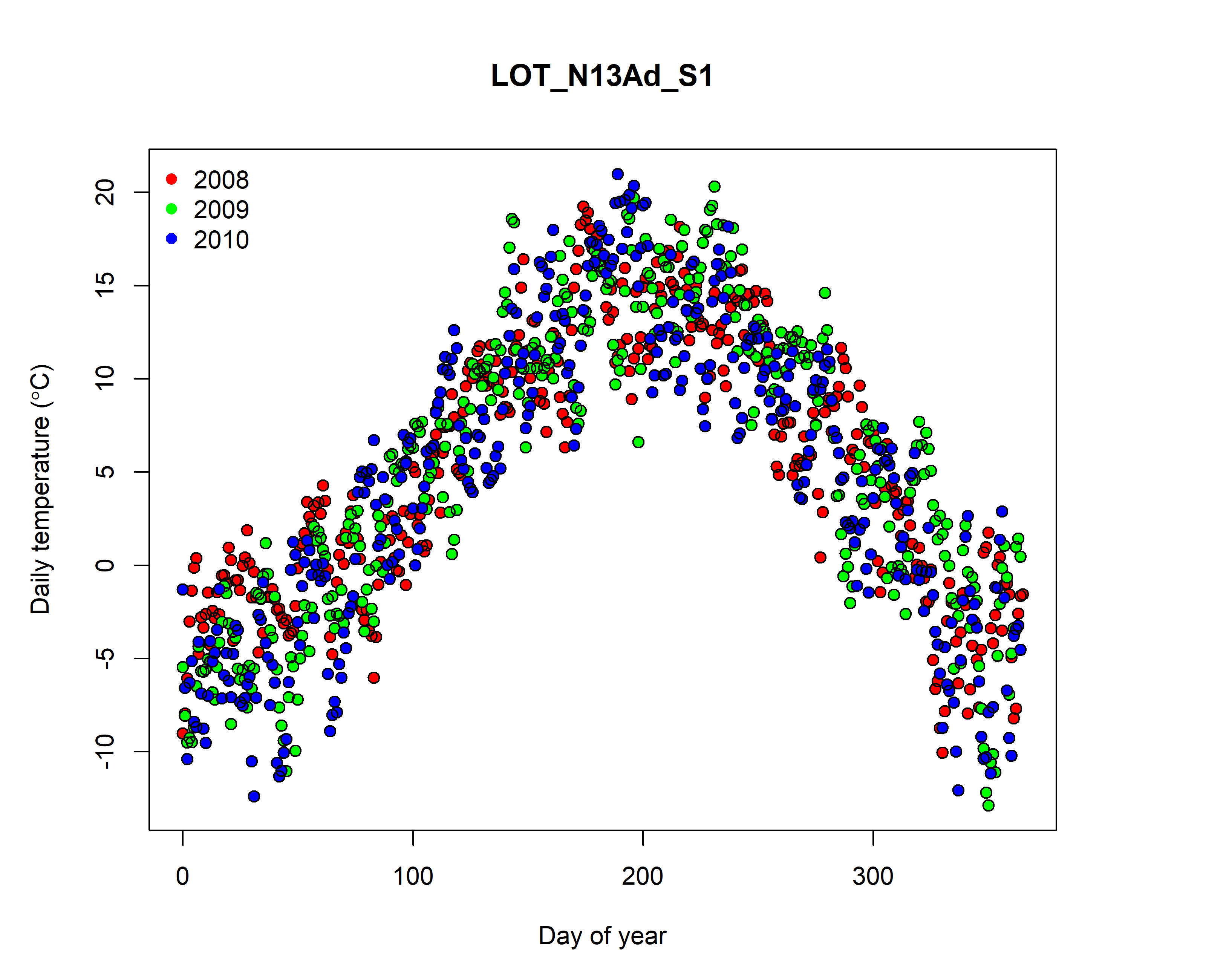
Figure: Here we plotted all three years of raw temperature data in the Lötschental (LOT; Switzerland). See Pappas et al. (2020; Ecography) for more site specific information.

4. Time-alignment (L1)

After converting the data into the correct format, it has to be time-aligned to regular time intervals with the function proc_L1. The resulting time resolution can be specified with the argument reso (in minutes, i.e. reso = 10 for a 10-minute resolution). Temperature data needs to be time-aligned in the same way as the dendrometer data.

Time-align dendrometer data with a 60 minute resolution (time zone is Greenwich Mean Time = GMT):

# suppress warnings
options(warn = -1)

# see help
?treenetproc::proc_L1	

# align data
dendro_data_L1 <- proc_L1(data_L0 = dendro_data_L0,
                          reso = 60, 
                          date_format ="%Y-%m-%d %H:%M:%S",
                          tz = "GMT")
head(dendro_data_L1)

##                    ts       series value version
## 1 2008-01-01 00:00:00 LOT_N13Ad_S1   415   0.1.4
## 2 2008-01-01 01:00:00 LOT_N13Ad_S1   422   0.1.4
## 3 2008-01-01 02:00:00 LOT_N13Ad_S1   418   0.1.4
## 4 2008-01-01 03:00:00 LOT_N13Ad_S1   414   0.1.4
## 5 2008-01-01 04:00:00 LOT_N13Ad_S1   417   0.1.4
## 6 2008-01-01 05:00:00 LOT_N13Ad_S1   414   0.1.4

Similar procedure for the temperature data:

# align data
temp_data_L1 <- proc_L1(data_L0 = temp_data_L0,
                        reso = 60,
                        date_format ="%Y-%m-%d %H:%M:%S", 
                        tz = "GMT")

The L1 data objects are now ready for error detection and processing.

5. Error detection and processing of the L1 data

Time-aligned dendrometer data can be cleaned and processed with the function proc_dendro_L2. To increase the quality of error detection, time-aligned temperature data is provided to temp_data_L1.

# see help
?treenetproc::dendro_data_L2

par(mfrow=c(1,1))
par(mar = c(5, 5, 5, 5))

# detect errors
dendro_data_L2 <- proc_dendro_L2(dendro_L1 = dendro_data_L1,
                                 temp_L1 = temp_data_L1, 
                                 plot = TRUE,
                                 tz="GMT")
# check the data
# head(dendro_data_L2)

## processing LOT_N13Ad_S1...
## No temperature data is missing.
## [1] "plot data..."

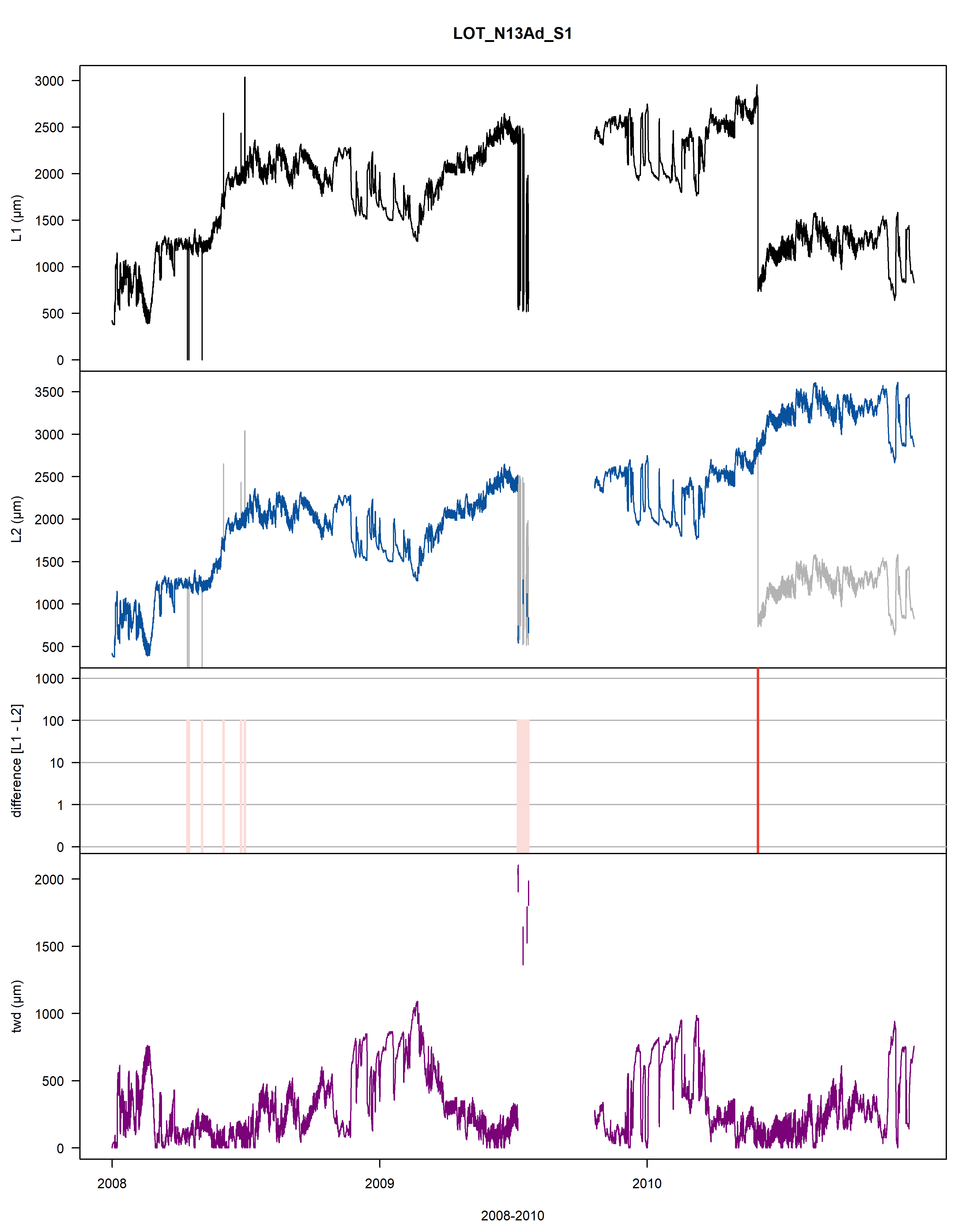
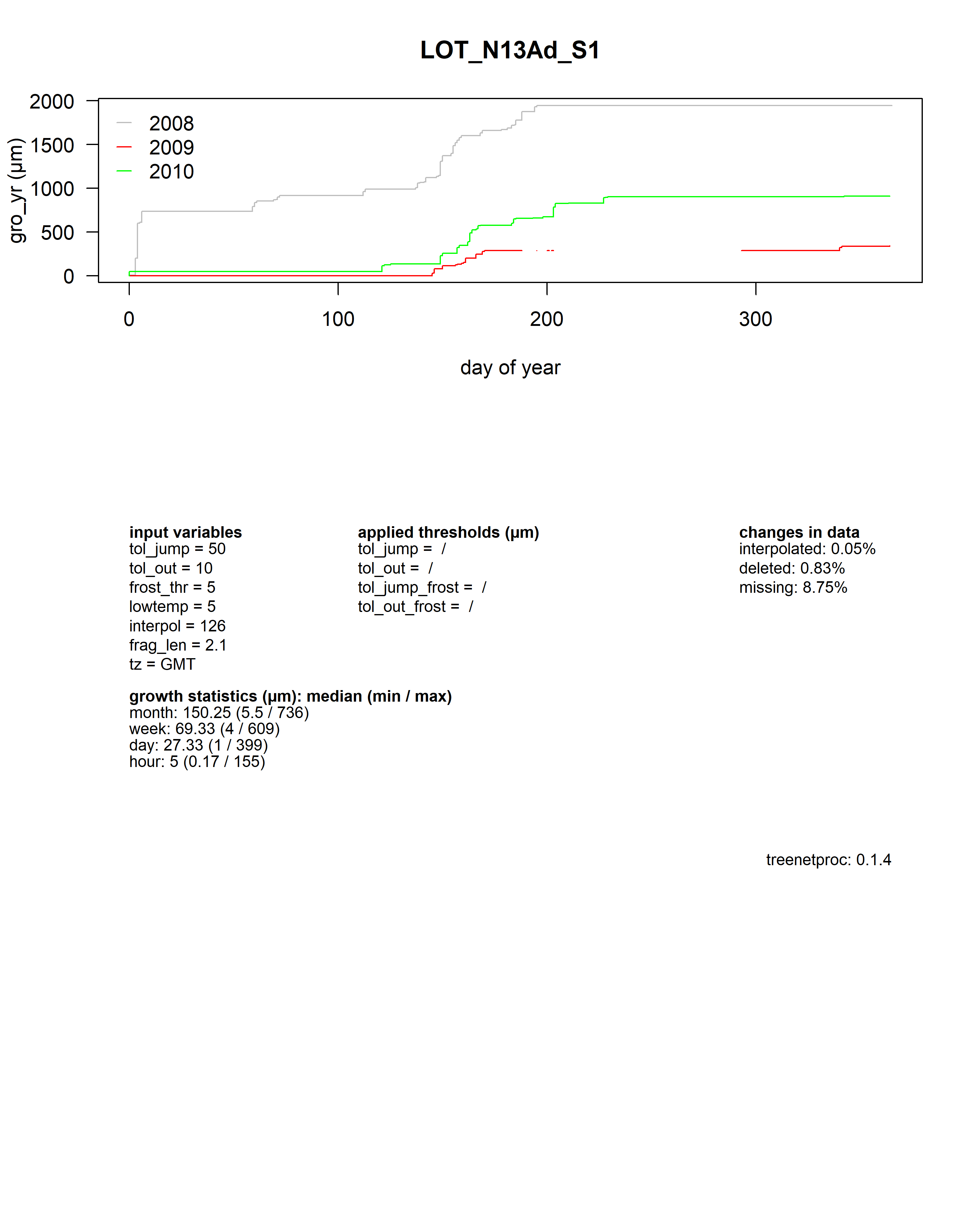
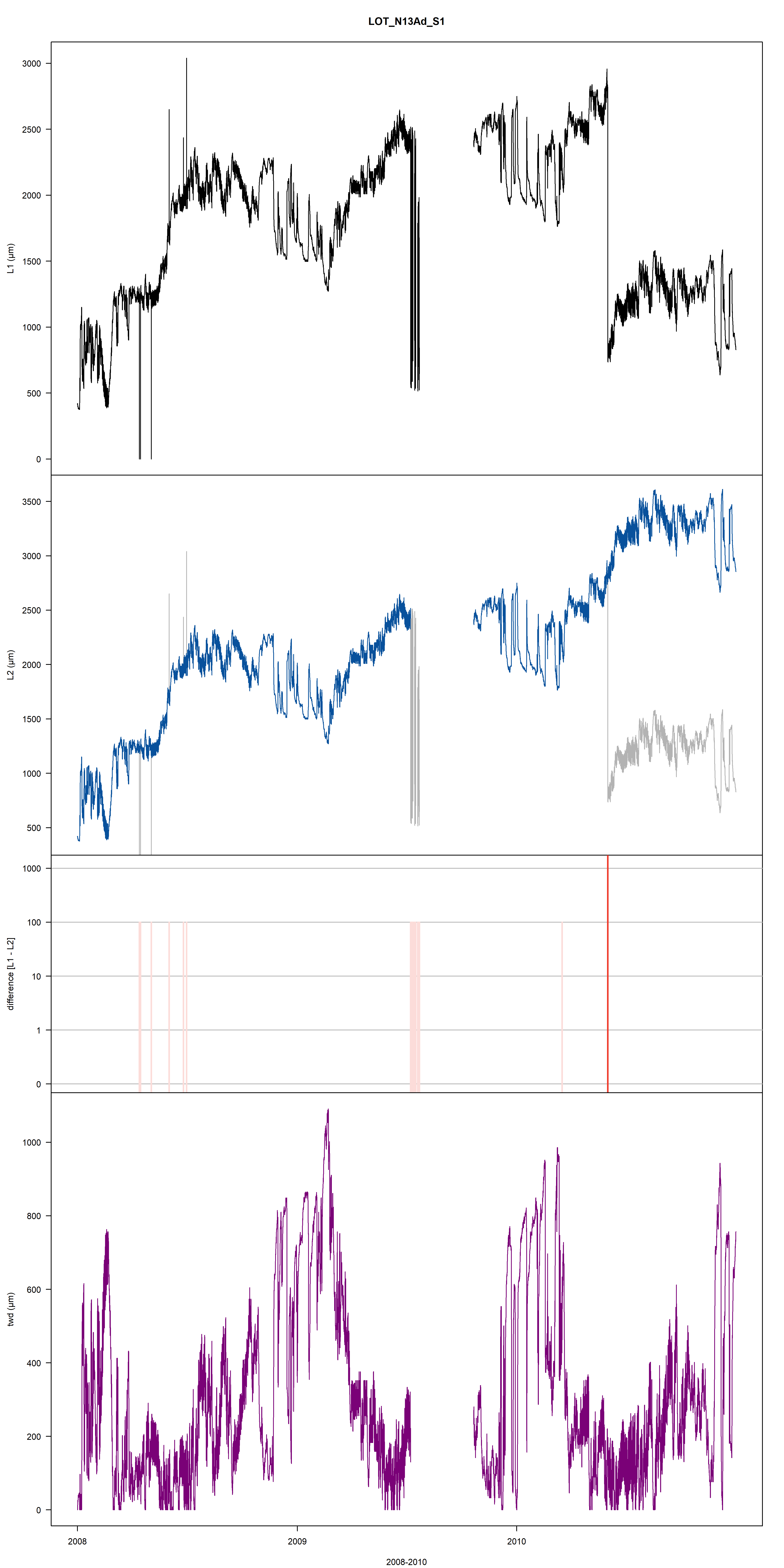
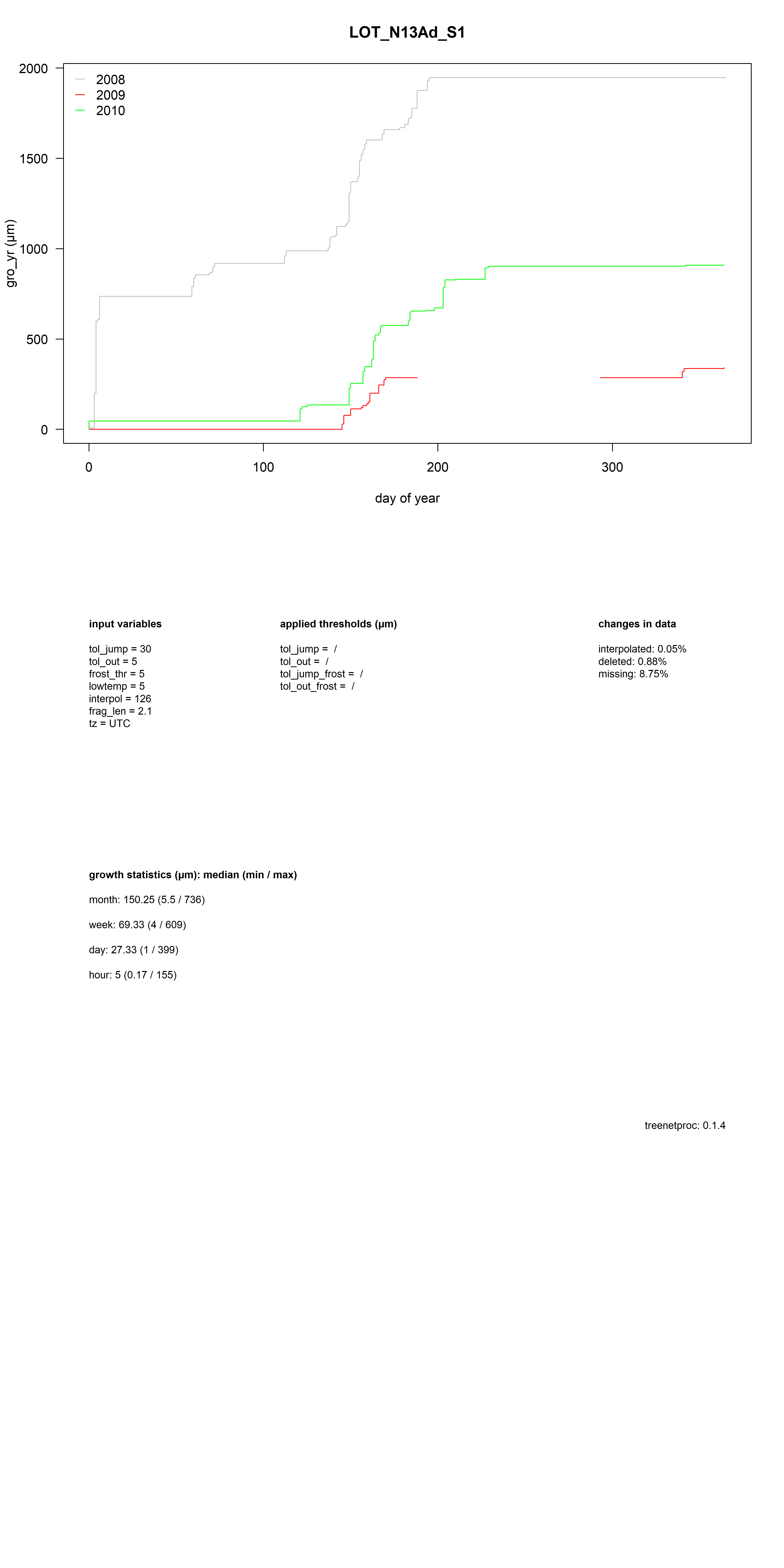
Figure: Visualisation plot of the function proc_dendro_L2. The first panel shows the stem radius changes of time-aligned dendrometer data (L1). The second panel shows cleaned L2 data. The third panel shows the data jump correction-induced differences between L1 and L2 data on a logarithmic scale. The fourth panel shows the tree-water deficit (twd). The final panel shows the annually accumulated growth curves (gro_yr).

A .pdf file is generated and saved on the working directory illustrating the outlier points and jumps that were corrected. Within this .pdf the first three plots illustrate the cleaning, while the last two provide information on the extracted tree water deficit (twd) and growth (gro_yr).

#highlight corrections made on the dendrometer data:
View(dendro_data_L2[which(is.na(dendro_data_L2$flags)==F),])

series	ts	value	max	twd	gro_yr	frost	flags	version
LOT_N13Ad_S1	2008-04-13 00:00:00	1219.000	1333	114.00000	918	TRUE	out1, fill	0.1.4
LOT_N13Ad_S1	2008-04-13 01:00:00	1223.000	1333	110.00000	918	TRUE	out1, fill	0.1.4
LOT_N13Ad_S1	2008-04-15 00:00:00	1267.333	1333	65.66667	918	TRUE	out1, fill	0.1.4
LOT_N13Ad_S1	2008-04-15 01:00:00	1268.667	1333	64.33333	918	TRUE	out1, fill	0.1.4
LOT_N13Ad_S1	2008-05-03 00:00:00	1232.667	1403	170.33333	988	TRUE	out1, fill	0.1.4
LOT_N13Ad_S1	2008-05-03 01:00:00	1236.333	1403	166.66667	988	TRUE	out1, fill	0.1.4
LOT_N13Ad_S1	2008-06-01 12:00:00	1661.000	1786	125.00000	1371	FALSE	out1, fill	0.1.4
LOT_N13Ad_S1	2008-06-01 13:00:00	1651.000	1786	135.00000	1371	FALSE	out1, fill	0.1.4
LOT_N13Ad_S1	2008-06-25 11:00:00	1942.000	2075	133.00000	1660	FALSE	out1, fill	0.1.4
LOT_N13Ad_S1	2008-06-25 12:00:00	1928.000	2075	147.00000	1660	FALSE	out1, fill	0.1.4
LOT_N13Ad_S1	2008-06-30 12:00:00	2048.333	2104	55.66667	1689	FALSE	out1, fill	0.1.4
LOT_N13Ad_S1	2008-06-30 13:00:00	2028.667	2104	75.33333	1689	FALSE	out1, fill	0.1.4
LOT_N13Ad_S1	2009-07-08 10:00:00	NA	NA	NA	NA	NA	out1	0.1.4
LOT_N13Ad_S1	2009-07-08 11:00:00	NA	NA	NA	NA	NA	out1	0.1.4
LOT_N13Ad_S1	2009-07-08 12:00:00	NA	NA	NA	NA	NA	out1	0.1.4
LOT_N13Ad_S1	2009-07-08 13:00:00	NA	NA	NA	NA	NA	out1	0.1.4
LOT_N13Ad_S1	2009-07-08 14:00:00	NA	NA	NA	NA	NA	out1	0.1.4
LOT_N13Ad_S1	2009-07-08 15:00:00	NA	NA	NA	NA	NA	out1	0.1.4
LOT_N13Ad_S1	2009-07-08 16:00:00	NA	NA	NA	NA	NA	out1	0.1.4
LOT_N13Ad_S1	2009-07-08 21:00:00	NA	NA	NA	NA	NA	out1	0.1.4
LOT_N13Ad_S1	2009-07-08 22:00:00	NA	NA	NA	NA	NA	out1	0.1.4
LOT_N13Ad_S1	2009-07-08 23:00:00	NA	NA	NA	NA	NA	out1	0.1.4
LOT_N13Ad_S1	2009-07-09 00:00:00	NA	NA	NA	NA	NA	out1	0.1.4
LOT_N13Ad_S1	2009-07-09 01:00:00	NA	NA	NA	NA	NA	out1	0.1.4
LOT_N13Ad_S1	2009-07-09 02:00:00	NA	NA	NA	NA	NA	out1	0.1.4

The column flags documents all changes that occurred during the error detection and processing. The numbers after the name of the flag specify in which iteration of cleaning process the changes occurred:

• "out": outlier point removed (e.g. “out1” for an outlier removed in iteration 1 of the cleaning process),
• "jump": jump corrected,
• "fill": value was linearly interpolated (length of gaps that are linearly interpolated can be specified with the argument interpol).

The visual checking of the results remains an essential step in dendrometer data cleaning. As mentioned all changes are plotted (plot = TRUE) and saved to a .pdf inf the current working directory (plot_export = TRUE). When plotted monthly (plot_period = "monthly"), each change to the data gets an ID. The ID numbers facilitate the reversal of wrong or unwanted corrections. Alternatively, the plots can be drawn for the full period (plot_period = "full") or for each year separately (plot_period = "yearly"). In these cases, the ID's are not displayed.

Here, we clean time-aligned (L1) dendrometer data and plot changes on a monthly resolution, in R (not exported to .pdf) for July 2009:

# create plot
par(mfrow=c(1,1))
par(mar = c(5, 5, 5, 5))

# grab a slice (one use one month instead of all)
dendro_data_L1_clip <- dendro_data_L1[which(left(dendro_data_L1$ts,7)=="2009-07"), ]

temp_data_L1_clip <- temp_data_L1[which(left(temp_data_L1$ts,7)=="2009-07"),]

# detect errors
dendro_data_L2_clip <- proc_dendro_L2(dendro_L1 = dendro_data_L1_clip,
               temp_L1 = temp_data_L1_clip,
               plot_period = "monthly", 
               plot_export = FALSE)
## processing LOT_N13Ad_S1...
## No temperature data is missing.
## [1] "plot data..."

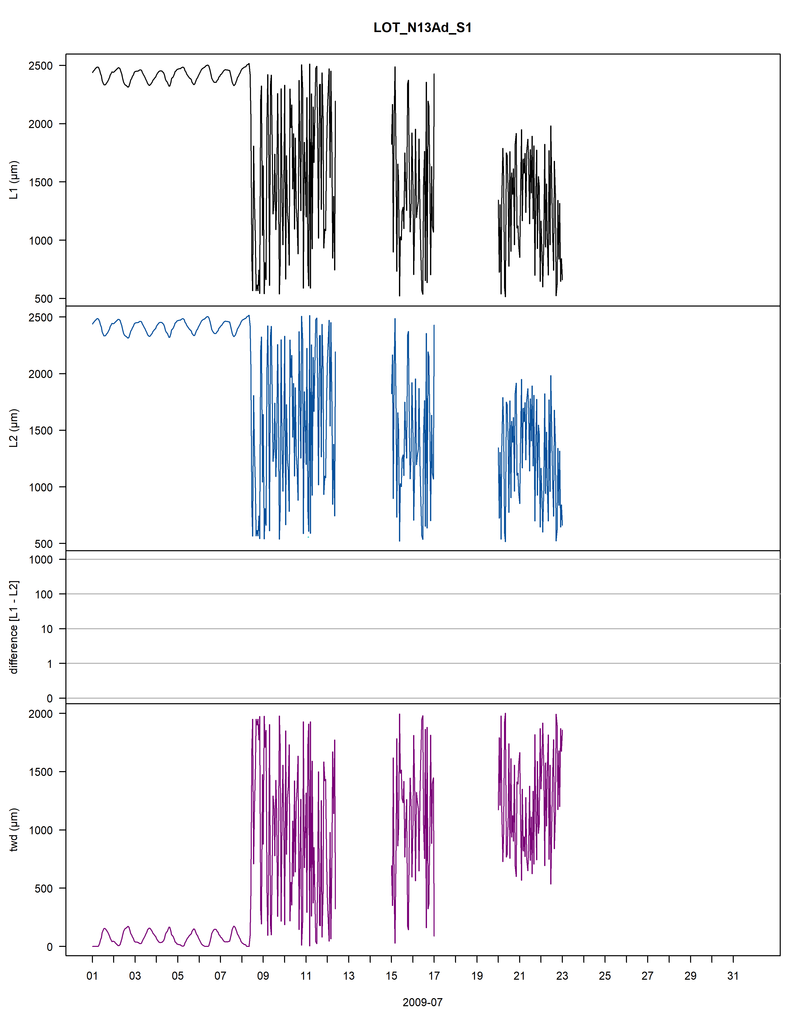
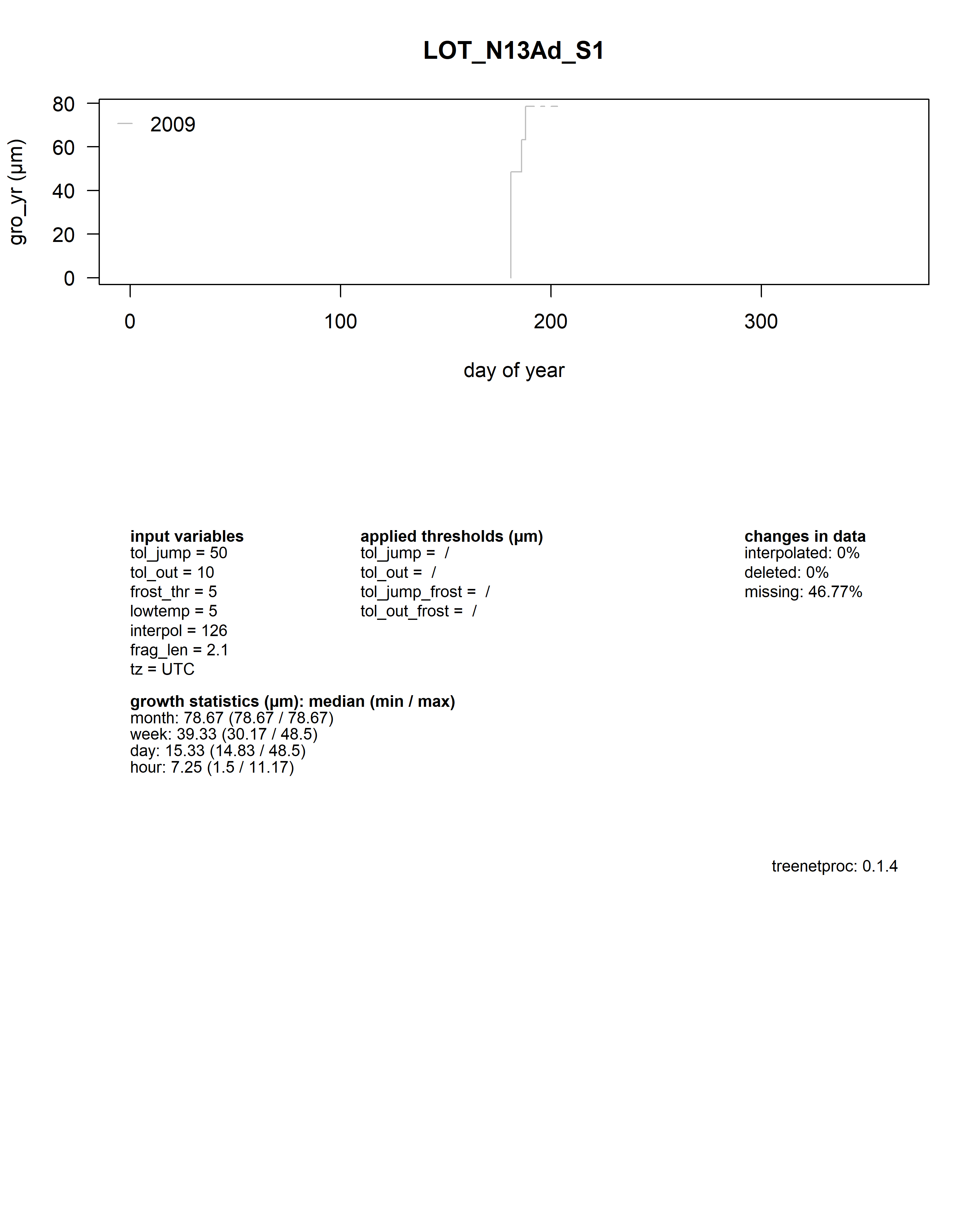
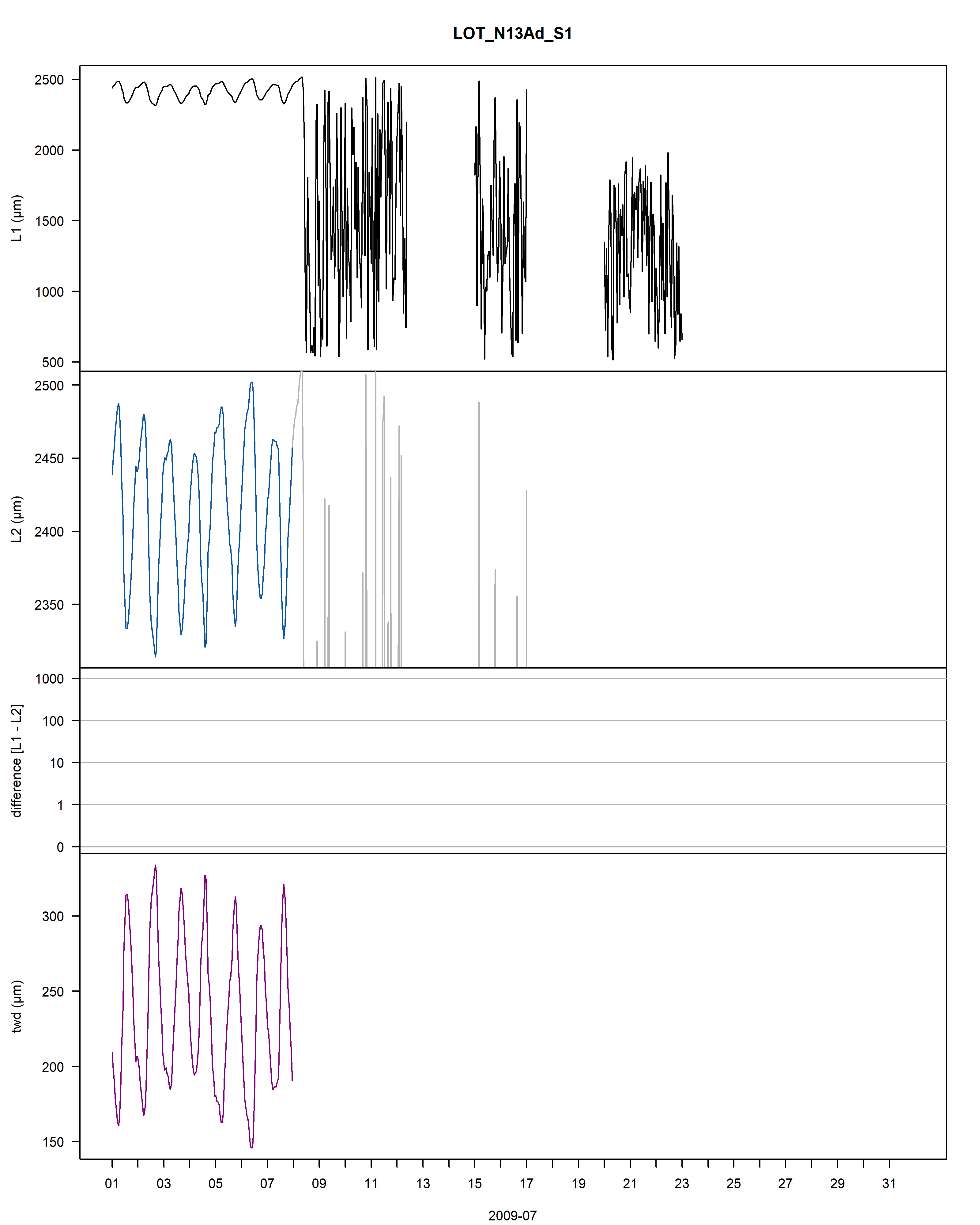
Figure: The plot contains an example of errors in the data, with 1) the stem radius changes of the raw time-aligned L1 dendrometer data in the first panel, 2) the stem radius changes of the cleaned L2 dendrometer data (with L1 data in the background in grey) in the second panel. Interpolated points are circled and frost periods are indicated with a horizontal, cyan line, 3) the changes between L1 and L2 data (red) as well as the deleted values (pink) in the third panel, 4) and the tree water deficit (twd) in the last panel.

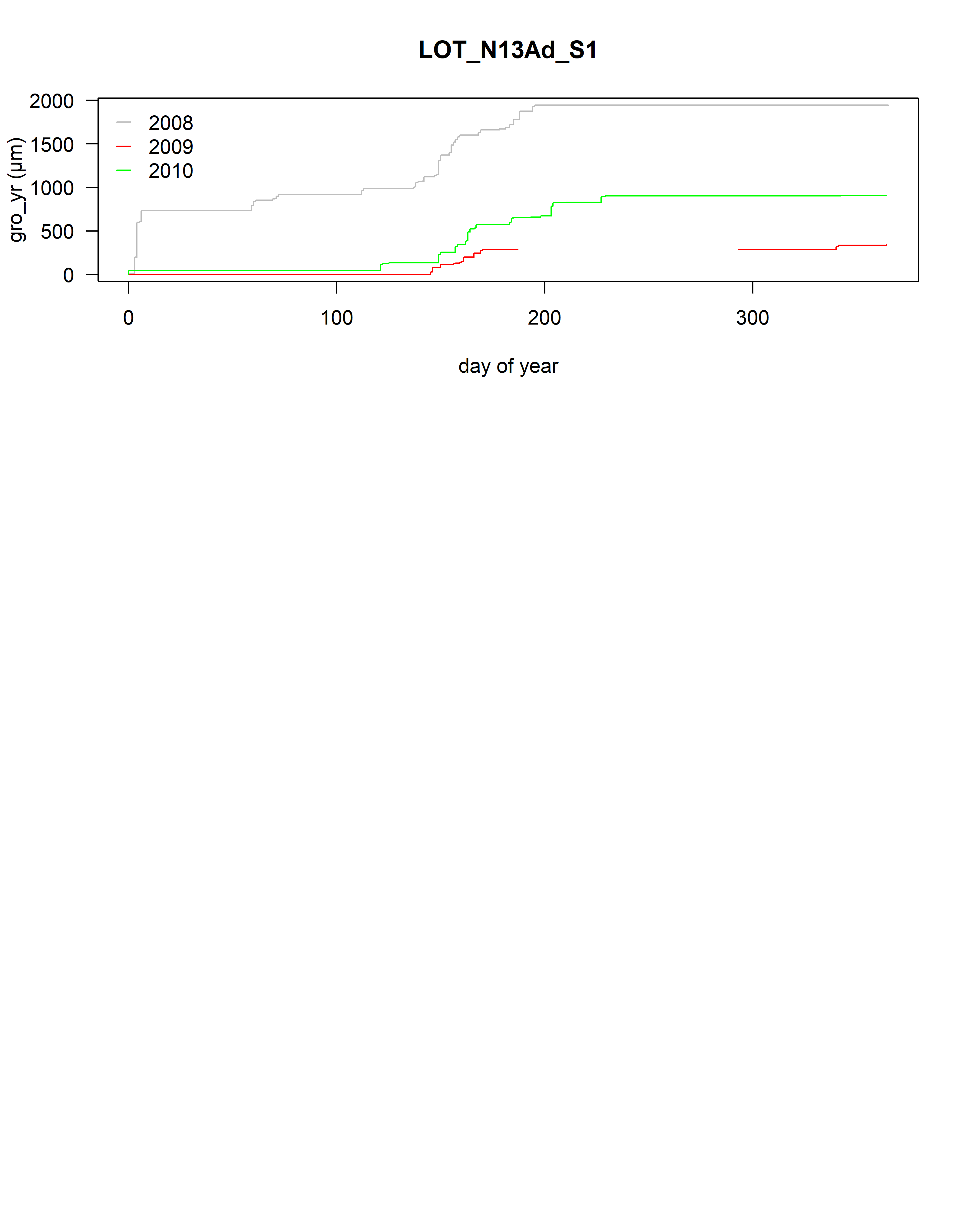
As a summary for each dendrometer series, an additional plot shows the yearly growth curves aligned by the day of year. Beneath the plot all input values, some growth statistics as well as the package version used are reported. When scrolling through to July 2009 (2009-07), one can see that although most of the errors (induced by sensor failure) have been removed some manual removing is still required.

Adjustments to parameters of proc_dendro_L2().

The rigidity of the error detection can be adjusted with the variables tol_out and tol_jump. Both variables control the thresholds used for the classification of outliers and jumps/shifts in the data. If values are erroneously deleted (i.e. classified as outliers), the value of tol_out should be increased (high values of tol_out decrease the rigidity of the thresholds).

Similarly, an increase in the value of tol_jump is needed if a dendrometer series is processed in a way that the original shape of the annual increment appears compressed (see example below).

# clean dendrometer data (tol_jump = 30, tol_out = 5):
par(mfrow=c(1,1))
par(mar = c(5, 5, 5, 5))

# detect errors
data_shrink_L2 <-proc_dendro_L2(dendro_L1 = dendro_data_L1,
                                temp_L1 = temp_data_L1,
                                tol_jump = 30,
                                tol_out = 5, 
                                plot_export = FALSE)
## processing LOT_N13Ad_S1...
## No temperature data is missing.
## [1] "plot data..."

When decreasing tol_out the function is able to remove outliers which were initially not detected (low values of tol_out increase the rigidity of the thresholds).

Providing temperature data

Providing temperature data along with dendrometer data ensures that frost and thaw events are not treated as outliers during data cleaning. In periods of probable frost (i.e. when the temperature < lowtemp) the threshold for outlier detection is multiplied by frost_thr.

If no temperature data is provided, a sample temperature dataset is used. The sample temperature dataset assumes potential frost and thaw conditions in the months December, January and February.

# processing w/o temperature data (using sample data set)
dendro_data_L2_notemp <- proc_dendro_L2(dendro_L1 = dendro_data_L1,
                                        tol_jump = 30, 
                                        tol_out = 5, 
                                        plot = FALSE)
## sample temperature dataset is used.
## processing LOT_N13Ad_S1...

# create plot
par(mfrow=c(1,1))
par(mar = c(5, 5, 5, 5))

plot(data = data_shrink_L2, 
     value ~ ts, 
     type = "n", 
     ylab = paste0("L2 (", "\u00b5", "m)"),
     las = 1)

lines(data = dendro_data_L1, value ~ ts, col = "grey70")
lines(data = dendro_data_L2_notemp, value ~ ts, col = "#08519c")

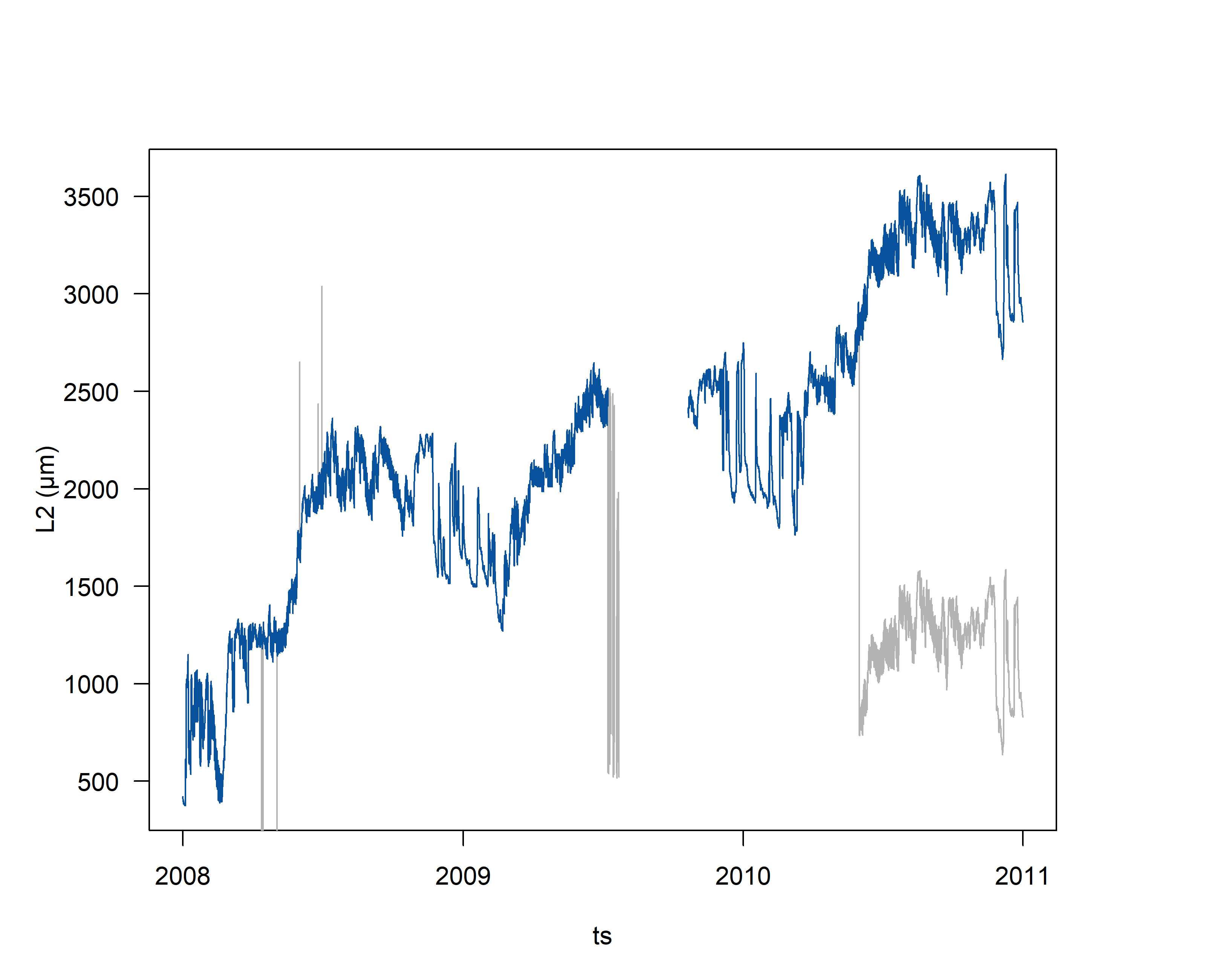
Figure: The sample temperature dataset does not assume frost after the end of February, therefore many values during the frost shrinkage are classified as outliers and deleted.

Manual corrections

Remaining errors that cannot be removed by adjusting the default values of tol_jump and/or tol_out can be corrected using the function corr_dendro_L2(). This function can be used to reverse erroneous changes or force changes that were not automatically made. There are three possibilities to manually correct remaining errors:

1. Reverse: specify the ID numbers of the changes that should be reversed. Remaining changes are renumbered starting at 1,
2. Force: force a shift in the data that was not corrected for by specifying a date up to five days prior to where the shift should occur,
3. Delete: delete an entire period of erroneous data by specifying a date range. This can also be done for L1 data with the function corr_dendro_L1().

# clean dendrometer data:
par(mfrow=c(1,1))
par(mar = c(5, 5, 5, 5))

dendro_data_L2 <- proc_dendro_L2(dendro_L1 = dendro_data_L1, 
                                 temp_L1 = temp_data_L1,
                                 plot_period = "monthly",
                                 plot_export = FALSE,
                                 tz="GMT")

# the code produces one plot per month!
# below is a sample plots from the correction procedure

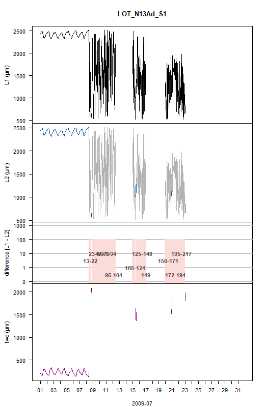
Figure: See previous examples above for detailed description.

The following error remained after data cleaning:

1. Not all erroneous data is removed in July 2009.

# correct data issue
# create plot
par(mfrow=c(1,1))
par(mar = c(5, 5, 5, 5))

dendro_data_L2<-corr_dendro_L2(dendro_L1 = dendro_data_L1, 
                               dendro_L2 = dendro_data_L2, 
                               delete = c("2009-07-08", "2009-07-24"),
                               series = "LOT_N13Ad_S1",
                               plot_export = FALSE,
                               tz="GMT")

dendro_data_L2[which((dendro_data_L2$flags)=="del"),]
## # A tibble: 385 x 9
##    series       ts                  value   max   twd gro_yr frost flags version
##    <fct>        <dttm>              <dbl> <dbl> <dbl>  <dbl> <lgl> <chr> <chr>  
##  1 LOT_N13Ad_S1 2009-07-08 00:00:00    NA    NA    NA     NA FALSE del   0.1.4  
##  2 LOT_N13Ad_S1 2009-07-08 01:00:00    NA    NA    NA     NA FALSE del   0.1.4  
##  3 LOT_N13Ad_S1 2009-07-08 02:00:00    NA    NA    NA     NA FALSE del   0.1.4  
##  4 LOT_N13Ad_S1 2009-07-08 03:00:00    NA    NA    NA     NA FALSE del   0.1.4  
##  5 LOT_N13Ad_S1 2009-07-08 04:00:00    NA    NA    NA     NA FALSE del   0.1.4  
##  6 LOT_N13Ad_S1 2009-07-08 05:00:00    NA    NA    NA     NA FALSE del   0.1.4  
##  7 LOT_N13Ad_S1 2009-07-08 06:00:00    NA    NA    NA     NA FALSE del   0.1.4  
##  8 LOT_N13Ad_S1 2009-07-08 07:00:00    NA    NA    NA     NA FALSE del   0.1.4  
##  9 LOT_N13Ad_S1 2009-07-08 08:00:00    NA    NA    NA     NA FALSE del   0.1.4  
## 10 LOT_N13Ad_S1 2009-07-08 09:00:00    NA    NA    NA     NA FALSE del   0.1.4  
## # ... with 375 more rows

Corrections are also reflected in the returned data.frame and all changes are documented in the column flags as:

1. "rev": for reversed corrections with the argument reverse,
2. "fjump": for forced jumps with the argument force,
3. "del": for deleted values with the argument delete.

6. Data Aggregation

Growing Season

After error detection and processing and the manual removal of remaining errors, the package offers two functions to calculate additional physiological parameters that may be of use for later analyses. The function grow_seas returns the day of year of growth onset and growth cessation.

# calculate growing season start and end:
?treenetproc::grow_seas

# aggregate to growing season by year
grow_seas_L2 <- grow_seas(dendro_L2 = dendro_data_L2,
                          agg_yearly=TRUE)
knitr::kable(grow_seas_L2, 
             caption = "Sample output data of the function `grow_seas`.")

series	year	gro_start	gro_end
LOT_N13Ad_S1	2009	147	342
LOT_N13Ad_S1	2010	1	228

The function returns a data.frame containing the day of year (doy) of the start and end of the growing season (see Table above). Values are returned starting from the second year only, since gro_start and gro_end depend on the values from the previous year. Notice the first year is not processed, since the calculation depends on the maximum dendrometer value of the previous year. To reduce the influence of potential remaining outliers on gro_start and gro_end, an adjustable tolerance tol_seas value is used to define growth start and cessation. This is clearly needed as 2010 shows a gro_start of 1.

# calculate growing season start and end with higher tol_seas 
# value of 0.1 (default = 0.05):
grow_seas_L2 <- grow_seas(dendro_L2 = dendro_data_L2, 
                          agg_yearly=TRUE,
                          tol_seas = 0.1)

knitr::kable(grow_seas_L2, 
             caption = "Sample output data of the function `grow_seas`.")

series	year	gro_start	gro_end
LOT_N13Ad_S1	2009	147	341
LOT_N13Ad_S1	2010	122	205

These results illustrate that the tree growth starts around the end of May, which is realistic for these species growing in the Alps. The asymptotic nature of the growth curves makes the definition of the end of the growing season more sensitive to tol_seas. Make sure to validate these numbers for rationality.

Phase statistics

Several characteristics of shrinkage and expansion phases can be calculated with the function phase_stats. The function phase_stats calculates the timing, duration, amplitude and the rate of change of shrinkage and expansion phases and outputs one plot per such phase. Below are two selected outputs from the function call (which produces > 3000 plots).

# calculate phase statistics

# see help
?treenetproc::phase_stats

# create plot
par(mfrow=c(1,1))
par(mar = c(5, 5, 5, 5))

phase_stats_L2 <- phase_stats(dendro_L2 = dendro_data_L2,
                              plot_phase = TRUE,
                              plot_export = TRUE)

## calculating phase statistics for LOT_N13Ad_S1...

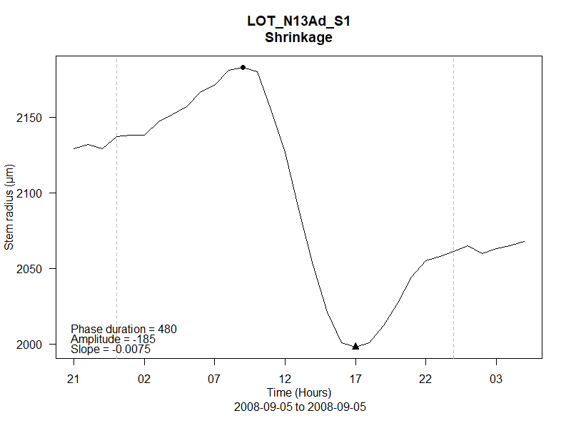
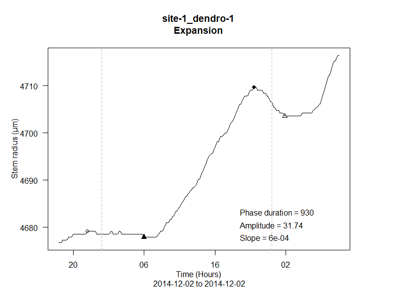
Figure: The plot shows the maximum (filled circle) and minimum (filled triangle) of the respective phase and reports its statistics. Empty circles and triangles show maxima or minima of previous or subsequent phases.

The function returns a data.frame containing the timing, duration, amplitude and slope of the shrinkage (shrink) and expansion (exp) phases. To evaluate the identification of shrinkage and expansion phases, all phases can be plotted by setting plot_phase = TRUE.

# view dalculated phase_stats:
knitr::kable(phase_stats_L2[1:5, ],
             caption = "Sample output data of the function `phase_stats`.")

series	day	doy	shrink_start	shrink_end	shrink_dur	shrink_amp	shrink_slope	exp_start	exp_end	exp_dur	exp_amp	exp_slope	phase_class
LOT_N13Ad_S1	2008-01-02	2	2008-01-01 22:00:00	2008-01-02 18:00:00	1200	-20	-0.0002457	2008-01-02 18:00:00	2008-01-02 23:00:00	300	8	0.0004841	-1
LOT_N13Ad_S1	2008-01-03	3	2008-01-02 23:00:00	2008-01-03 16:00:00	1020	-12	-0.0001691	NA	NA	NA	NA	NA	NA
LOT_N13Ad_S1	2008-01-04	4	NA	NA	NA	NA	NA	2008-01-03 16:00:00	2008-01-04 09:00:00	1020	5	0.0000338	NA
LOT_N13Ad_S1	2008-01-04	4	NA	NA	NA	NA	NA	2008-01-04 13:00:00	2008-01-04 21:00:00	480	239	0.0104537	NA
LOT_N13Ad_S1	2008-01-05	5	2008-01-04 21:00:00	2008-01-05 05:00:00	480	-97	-0.0036852	NA	NA	NA	NA	NA	NA

Such information could be used to identifies days on which radial change is likely driven by transpiration (phase_class = 1) or temperature (phase_class = -1).

# calculate radial change patterns:
options(warn = 1)

trans_stats_L2 <- phase_stats_L2[which(phase_stats_L2$phase_class==1),]
temp_stats_L2 <- phase_stats_L2[which(phase_stats_L2$phase_class==-1),]
other_stats_L2 <- phase_stats_L2[which(is.na(phase_stats_L2$phase_class)==T),]
other_stats_L2$phase_class <- 0

trans <- aggregate(trans_stats_L2$phase_class,by=list(trans_stats_L2$doy),sum)
temp <- aggregate(temp_stats_L2$phase_class,by=list(temp_stats_L2$doy),sum)
temp$x <- sqrt(temp$x^2)
other <- aggregate(other_stats_L2$phase_class,by=list(other_stats_L2$doy),sum)

# plot causes of daily radial change patterns:
par(mfrow=c(1,1))
par(mar = c(5, 5, 5, 5))

plot(trans$Group.1,trans$x,
     pch=16,
     col="black",
     cex=2,
     ylim=c(0,4),
     ylab="Cumulative days",
     xlab="Day of year")

points(trans$Group.1,trans$x,pch=16,cex=1,col="cyan")
points(temp$Group.1,temp$x,pch=16,cex=2,col="black")
points(temp$Group.1,temp$x,pch=16,cex=1,col="darkorange")
points(other$Group.1,other$x,pch=16,cex=2,col="black")
points(other$Group.1,other$x,pch=16,cex=1,col="grey70")

legend("topleft",
       pch=16,
       c("Transpiration","Temperature","Other"),
       col=c("cyan","darkorange","grey70"),
       bty="n",
       pt.cex=1.5,
       cex=1.5)

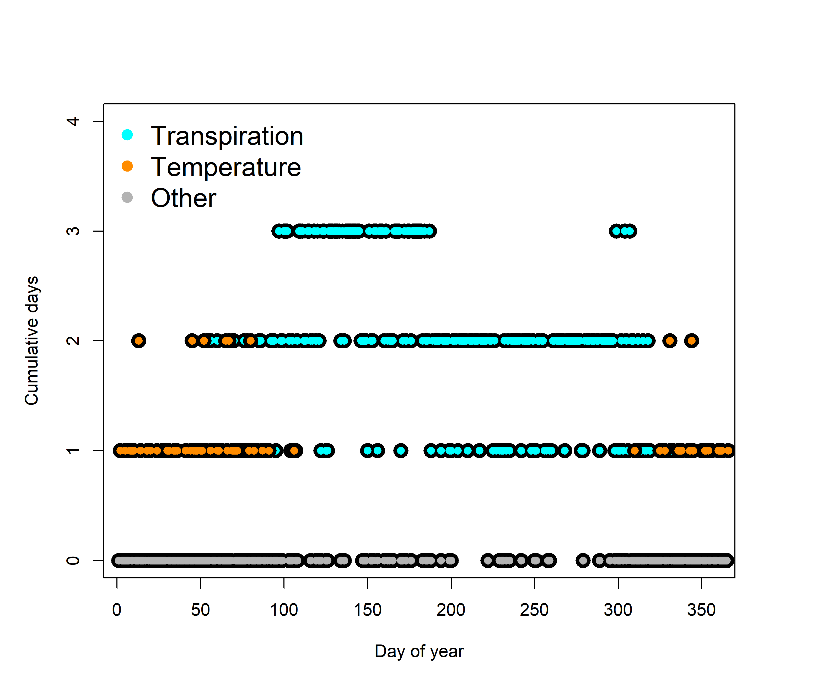
Figure: Cumulative days of the three years (2008, 2009 and 2010) where the daily cycle is likely explained by transpiration, temperature or something else (other). These results show that transpiration for this individual tree is starting around day of year 50 and continues until day of year 325.

Tree water deficit (TWD) as an indicator of drought stress.

# plot minimum daily twd against day of year
par(mfrow=c(1,1))
par(mar = c(5, 5, 5, 5))

plot(1,
     1,
     ylim=c(0,max(dendro_data_L2$twd,na.rm=T)),
     xlim=c(0,365),
     ylab=expression("twd ("*mu*"m)"),
     xlab="Day of year",
     col="white")

col_sel<-c("cyan","darkorange","purple")

for(y in c(1:length(unique(left(dendro_data_L2$ts,4))))){
  # selected year
  sel<-dendro_data_L2[which(left(dendro_data_L2$ts,4)==unique(left(dendro_data_L2$ts,4))[y]),]
  # calc twd
  twd<-suppressWarnings(aggregate(sel$twd,list(as.Date(sel$ts)),min,na.rm=T))
  twd$doy<-as.numeric(strftime(as.Date(twd$Group.1), format = "%j"))
  
  # clean
  twd[which(twd$x=="Inf"),"x"]<-NA
  
  lines(twd$doy,twd$x,col=col_sel[y],lwd=1.5)
  twd[which(is.na(twd$x)==T),"x"]<-0
  polygon(c(c(0,twd$doy),c(rev(twd$doy),0)),
          c(c(0,twd$x),rep(0,nrow(twd)+1)),
          col=rgb(0,0,0,0.1),
          border=rgb(0,0,0,0))
}

legend("topleft",
       c(unique(left(dendro_data_L2$ts,4))),
       col=col_sel,
       lty=1,
       bty="n")

# Add growing season extent:
grow_seas_L2 <- grow_seas(dendro_L2 = dendro_data_L2,
                          agg_yearly=TRUE,
                          tol_seas = 0.1)


abline(v=c(mean(grow_seas_L2$gro_start),
           mean(grow_seas_L2$gro_end)),
       lty=2)
text(mean(c(mean(grow_seas_L2$gro_start),
            mean(grow_seas_L2$gro_end))),
     max(dendro_data_L2$twd,na.rm=T),
     "Growing season")

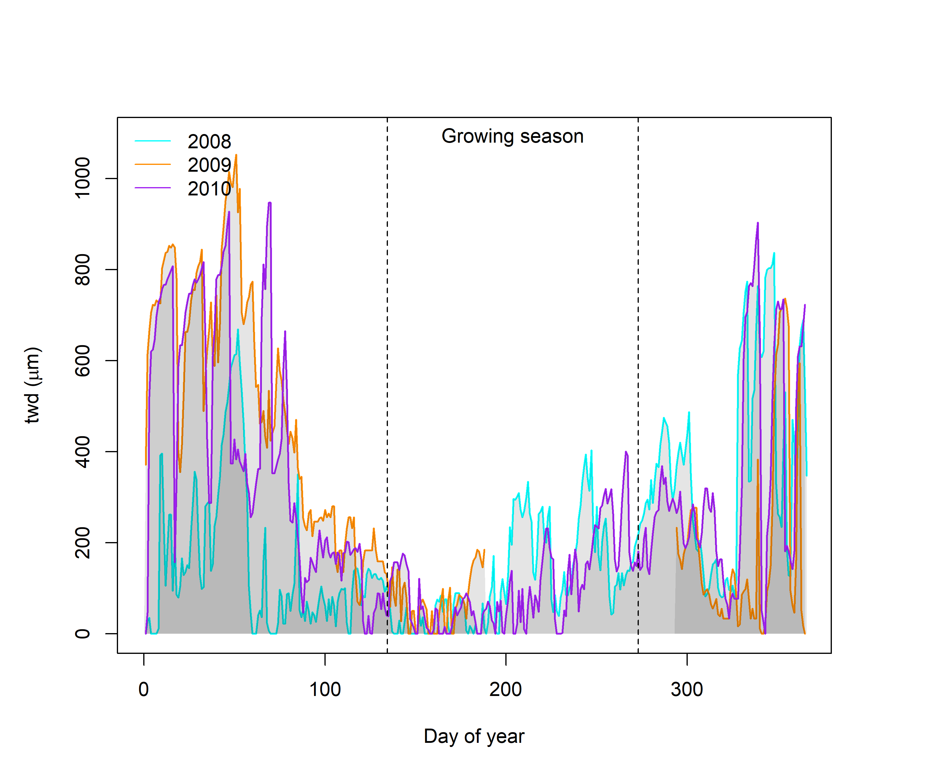
Figure: Tree water deficit (TWD) dynamics reveal that the tree mainly shrinks during the night in winter. Besides winter shrinkage, drought impacts should be detected within the growing season. During the growing season 2008 showed more shrinkage compared to 2010, revealing the tree was experience stronger water limitation during growth.

7. Using treeprocnet

For use in publication, the reference is:

citation("treenetproc")
## 
## To cite treenetproc in publications use:
## 
##   Knüsel S., Haeni M., Wilhelm M., Peters R.L., Zweifel R. 2020.
##   treenetproc: towards a standardized processing of stem radius data.
##   In prep.
## 
##   Haeni M., Knüsel S., Wilhelm M., Peters R.L., Zweifel R. 2020.
##   treenetproc - Clean, process and visualise dendrometer data. R
##   package version 0.1.4. Github repository:
##   https://github.com/treenet/treenetproc
## 
##   Hadley Wickham, Romain François, Lionel Henry and Kirill Müller
##   (2019). dplyr: A Grammar of Data Manipulation. R package version
##   0.8.3. https://CRAN.R-project.org/package=dplyr
## 
## To see these entries in BibTeX format, use 'print(<citation>,
## bibtex=TRUE)', 'toBibtex(.)', or set
## 'options(citation.bibtex.max=999)'.

8. References

• Pappas C, Peters RL, Fonti P (2020) Linking variability of tree water use and growth with species resilience to environmental changes. Ecography. 43: 1-14.
• Knüsel S, Haeni M, Wilhelm M, Peters RL, Zweifel R (2020) treenetproc: towards a standardized processing of stem radius data. In prep.
• Zweifel R, Haeni M, Buchmann N, Eugster W (2016) Are trees able to grow in periods of stem shrinkage? New Phytol. 211:839-49.

See also:

• treenetproc package vignette
• The Lötschental tree-growth monitoring transect

9. Contact

For questions, please get in touch with Richard Peters