Using treenetproc to process Hyytiälä dendrometer data
1. Background
The dendrometer data cleaned with datacleanr can be used to assess both drought stress and growth patterns. Within the example we will process the dendrometer data using the treenetproc R package. We will use the package on a Scots pine and birch tree to analyze the differences in growth patterns and water stress levels. A step by step example is provided on how to process the dendrometer data. Then concrete questions will be asked in relation to the species.
The package treenetproc cleans, processes and visualizes highly resolved time series of dendrometer data in two steps; raw dendrometer data is aligned to regular time intervals (level 1: L1) and cleaned (level 2: L2).
In an optional third step several commonly used characteristics such as the start and end of stem growth can be calculated.
This tutorial presents an example for processing two dendrometer time-series, yet the package does allow for processing of multiple time-series in one run.
2. Set-up Steps
# install if necessary
packages <- (c("devtools","zoo","chron","dplyr","viridis", "RCurl", "DT"))
install.packages(setdiff(packages, rownames(installed.packages())))


devtools::install_github("treenet/treenetproc")

library(treenetproc)
library(zoo)
library(chron)
library(viridis)
library(dplyr)

# helper functions
left <-  function(string, char){substr(string, 1,char)}
right <-  function (string, char){substr(string,nchar(string)-(char-1),nchar(string))}
##
## Attaching package: 'zoo'
## The following objects are masked from 'package:base':
##
##     as.Date, as.Date.numeric
## Loading required package: viridisLite
##
## Attaching package: 'dplyr'
## The following objects are masked from 'package:stats':
##
##     filter, lag
## The following objects are masked from 'package:base':
##
##     intersect, setdiff, setequal, union
3. Import data (L0)
Raw dendrometer and temperature data can be provided as input. Providing temperature data is optional. However, temperature data increases the quality of error detection and processing.
The raw dendrometer or climate data can be provided in long format. Data of multiple sensors can either be specified in a column named series to separate the sensors.
Dendrometer data always has to be provided in microns.
In addition, a column named ts with timestamps in any standard date format (default is date_format = "%Y-%m-%d %H:%M:%S") is required.
Dendrometer data:
Find an example data set to download and place in your current working directory here:
# set you working directory on the correct path!
#[click: Session -> Select Working Directory -> Choose Directory; or change to below provided code]
 # setwd("D:/Documents/UL - POSTDOC/02_communication/Education - Finland/Course - Data")

# import table cleaned with datacleanr
dendro_data_L0<-readRDS("dendrometer_cleaned.Rds")
dendro_data_L0<-as.data.frame(dendro_data_L0)
colnames(dendro_data_L0)[1]<-"ts"
colnames(dendro_data_L0)[2]<-"series"
dendro_data_L0<-dendro_data_L0[,c(2,1,3)]

# to simplify the analyses we pick one Scots pine tree and one birch tree
dendro_data_L0<-dendro_data_L0[which(dendro_data_L0$series!="dendro_stem_pine_Sylvib_LVDT"),]

# moreover, values in January are removed to ease the annual analyses
dendro_data_L0[which(right(left(dendro_data_L0$ts,7),2)[1]=="01"),]$value<-NA

# this script requires positive values and due to re-installment during the winter we need to shift each year to the value of the previous years maximum (this assures that each year is analyzed independently from the previous years values)
sensors<-unique(dendro_data_L0$series)
years<-left(dendro_data_L0$ts,4)
for(s in c(1:length(sensors))){
    for(y in c(1:length(unique(years)))){
if(y==1){correction<-0}else{
    correction<-max(dendro_data_L0[which(dendro_data_L0$series==sensors[s]&years==unique(years)[y-1]),]$value,na.rm=T)
    }
initial<-na.omit(dendro_data_L0[which(dendro_data_L0$series==sensors[s]&years==unique(years)[y]),]$value)[1]
dendro_data_L0[which(dendro_data_L0$series==sensors[s]&years==unique(years)[y]),]$value<-
dendro_data_L0[which(dendro_data_L0$series==sensors[s]&years==unique(years)[y]),]$value-initial+correction
}
}

# Illustrate the structure of the input data:
str(dendro_data_L0)
## 'data.frame':	381650 obs. of  3 variables:
##  $ series: chr  "dendro_stem_pine_Jennib_LVDT" "dendro_stem_pine_Jennib_LVDT" "dendro_stem_pine_Jennib_LVDT" "dendro_stem_pine_Jennib_LVDT" ...
##  $ ts    : POSIXct, format: "2015-01-01 00:00:00" "2015-01-01 00:10:00" ...
##  $ value : num  NA NA NA NA NA NA NA NA NA NA ...

# Table structure:
head(dendro_data_L0)
##                         series                  ts value
## 1 dendro_stem_pine_Jennib_LVDT 2015-01-01 00:00:00    NA
## 2 dendro_stem_pine_Jennib_LVDT 2015-01-01 00:10:00    NA
## 3 dendro_stem_pine_Jennib_LVDT 2015-01-01 00:20:00    NA
## 4 dendro_stem_pine_Jennib_LVDT 2015-01-01 00:30:00    NA
## 5 dendro_stem_pine_Jennib_LVDT 2015-01-01 00:40:00    NA
## 6 dendro_stem_pine_Jennib_LVDT 2015-01-01 00:50:00    NA

# one can see that there is an error in the label as Jennib is a birch tree which needs to be changed
dendro_data_L0[which(dendro_data_L0$series=="dendro_stem_pine_Jennib_LVDT"),]$series<-"dendro_stem_birch_Jennib_LVDT"
unique(dendro_data_L0$series)
## [1] "dendro_stem_birch_Jennib_LVDT" "dendro_stem_pine_Penttib_LVDT"
Multiple data issues are present within the data, including a measurement jump due to re-installing the sensor in 2016.
4. Time-alignment (L1)
After converting the data into the correct format, it has to be time-aligned to regular time intervals with the function proc_L1.
The resulting time resolution can be specified with the argument reso (in minutes, i.e. reso = 10 for a 10-minute resolution).
Time-align dendrometer data with a 60 minute resolution (time zone is set for simplicity to Coordinated Universal Time = UTC):
# suppress warnings
options(warn = -1)

# see help
?treenetproc::proc_L1
## starting httpd help server ... done

# align data
dendro_data_L1 <- proc_L1(data_L0 = dendro_data_L0,
                          reso = 60,
                          date_format ="%Y-%m-%d %H:%M:%S",
                          tz = "UTC")
head(dendro_data_L1)
##                    ts                        series value version
## 1 2015-01-01 00:00:00 dendro_stem_birch_Jennib_LVDT    NA   0.1.4
## 2 2015-01-01 01:00:00 dendro_stem_birch_Jennib_LVDT    NA   0.1.4
## 3 2015-01-01 02:00:00 dendro_stem_birch_Jennib_LVDT    NA   0.1.4
## 4 2015-01-01 03:00:00 dendro_stem_birch_Jennib_LVDT    NA   0.1.4
## 5 2015-01-01 04:00:00 dendro_stem_birch_Jennib_LVDT    NA   0.1.4
## 6 2015-01-01 05:00:00 dendro_stem_birch_Jennib_LVDT    NA   0.1.4
The L1 data objects are now ready for error detection and processing.
5. Error detection and processing of the L1 data
Time-aligned dendrometer data can be cleaned and processed with the function proc_dendro_L2.
# see help
?treenetproc::dendro_data_L2

# detect errors
dendro_data_L2 <- proc_dendro_L2(dendro_L1 = dendro_data_L1,
                                 plot = TRUE,
                                 tz="UTC")
## sample temperature dataset is used.
## processing dendro_stem_birch_Jennib_LVDT...
## processing dendro_stem_pine_Penttib_LVDT...
## [1] "plot data..."

# check the data that is presented in a pdf in your working directory

# see the data structure
head(dendro_data_L2)
## # A tibble: 6 x 9
##   series        ts                  value   max   twd gro_yr frost flags version
##   <chr>         <dttm>              <dbl> <dbl> <dbl>  <dbl> <lgl> <chr> <chr>
## 1 dendro_stem_~ 2015-01-01 00:00:00    NA    NA    NA     NA NA    <NA>  0.1.4
## 2 dendro_stem_~ 2015-01-01 01:00:00    NA    NA    NA     NA NA    <NA>  0.1.4
## 3 dendro_stem_~ 2015-01-01 02:00:00    NA    NA    NA     NA NA    <NA>  0.1.4
## 4 dendro_stem_~ 2015-01-01 03:00:00    NA    NA    NA     NA NA    <NA>  0.1.4
## 5 dendro_stem_~ 2015-01-01 04:00:00    NA    NA    NA     NA NA    <NA>  0.1.4
## 6 dendro_stem_~ 2015-01-01 05:00:00    NA    NA    NA     NA NA    <NA>  0.1.4
A .pdf file is generated and saved on the working directory illustrating the outlier points and jumps that were corrected.
Within this .pdf the first three plots illustrate the cleaning, while the last two provide information on the extracted tree water deficit (twd) and growth (gro_yr).
## sample temperature dataset is used.
## processing dendro_stem_birch_Jennib_LVDT...
## processing dendro_stem_pine_Penttib_LVDT...
## [1] "plot data..."
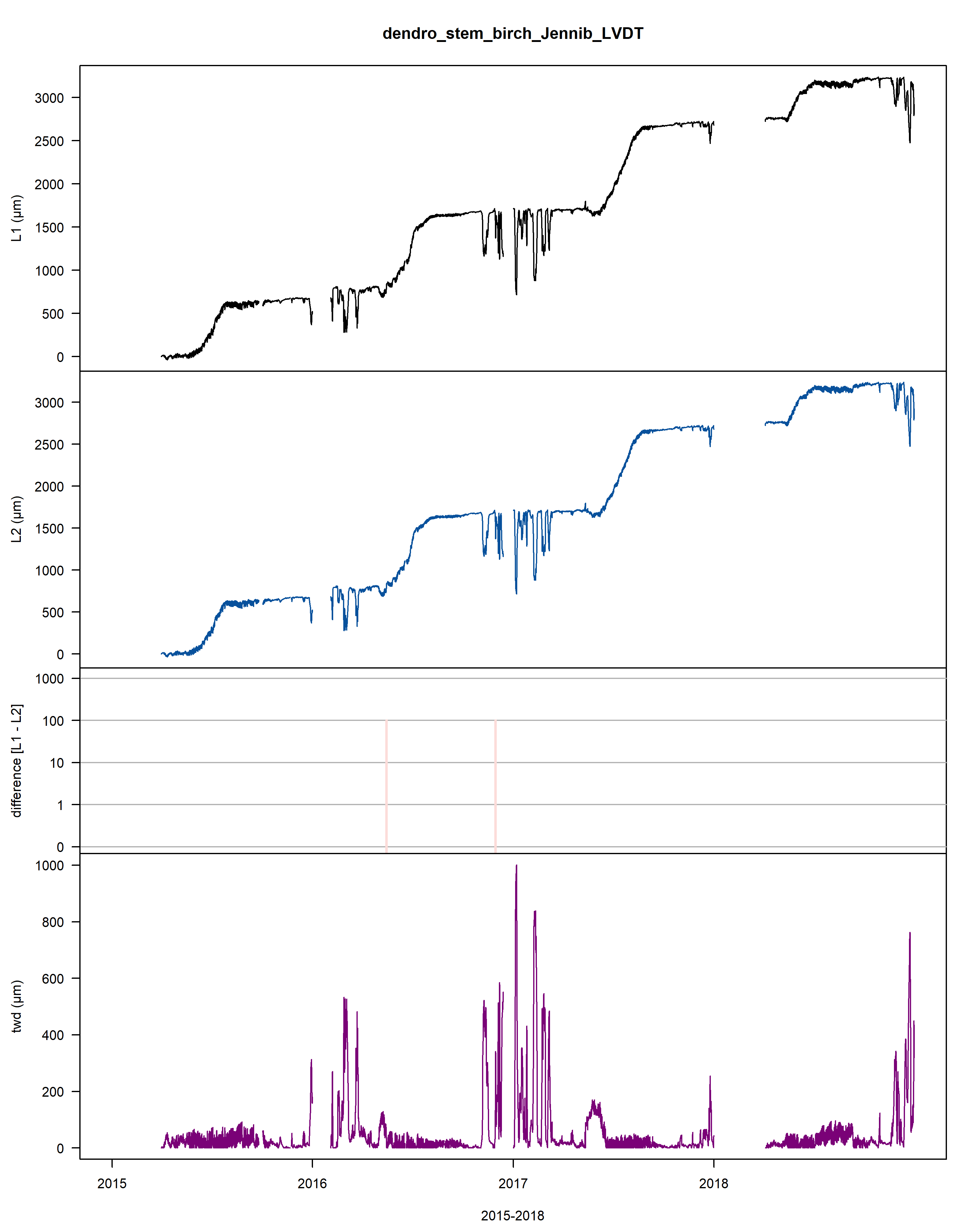
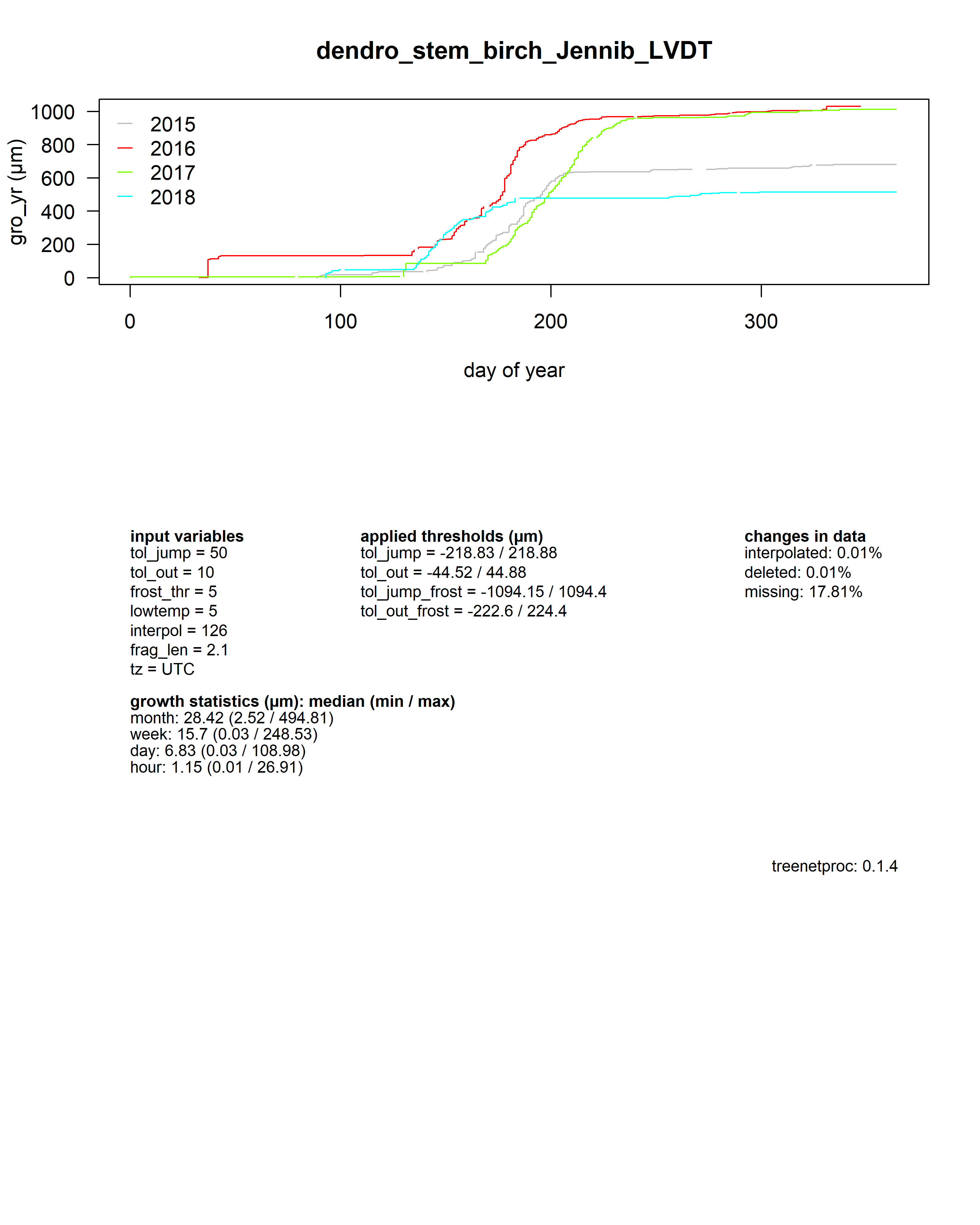
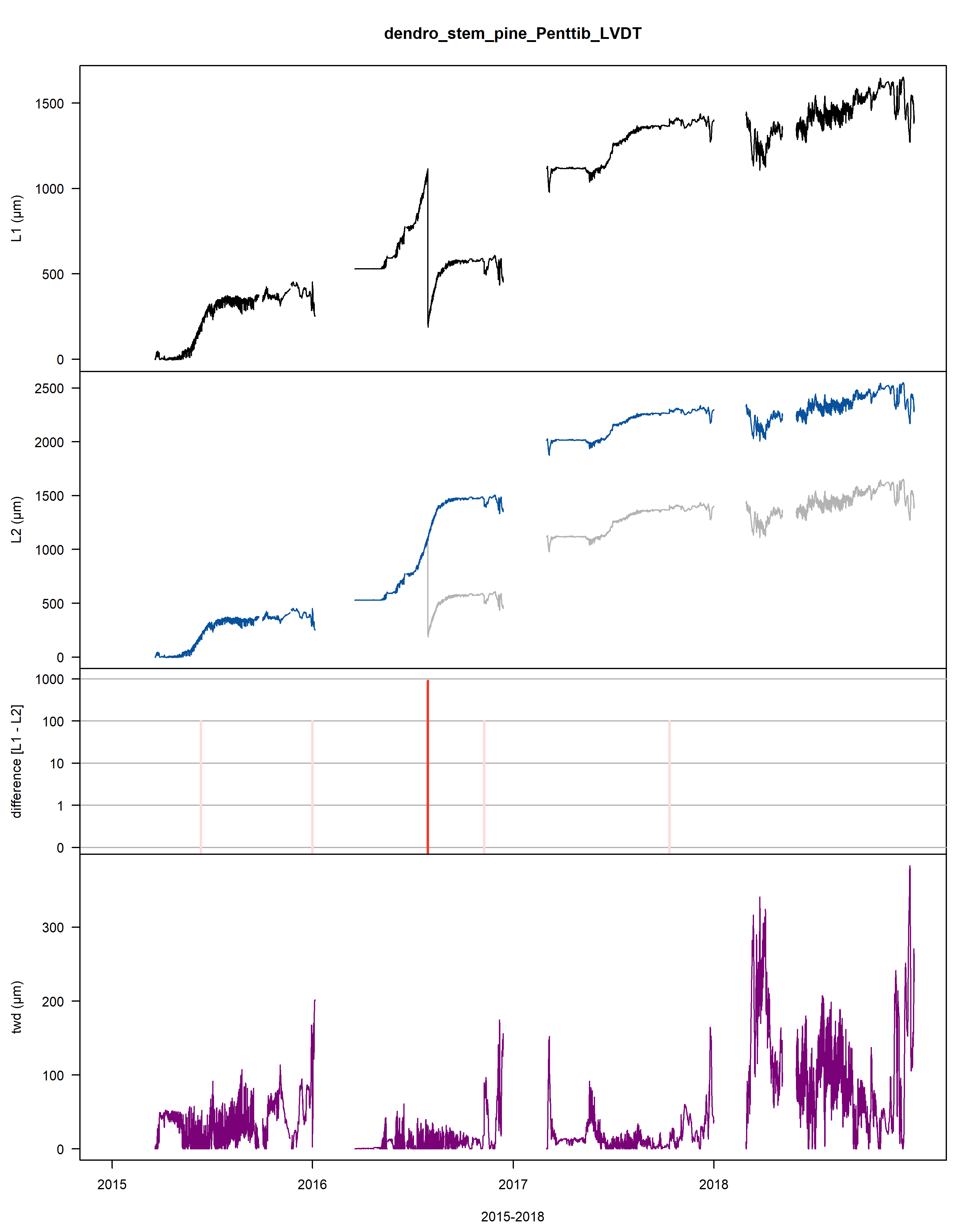
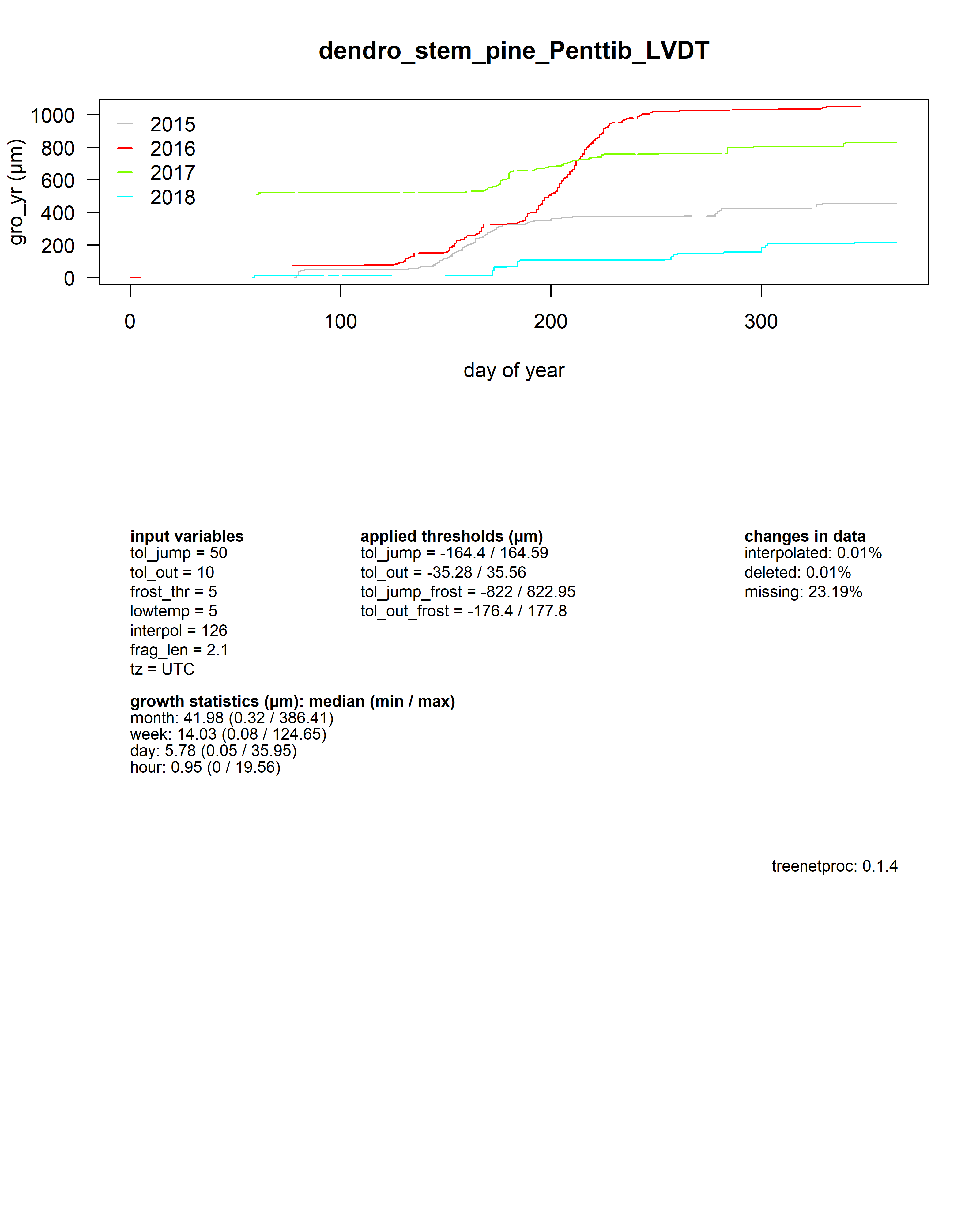
Figure: Visualisation plot of the function proc_dendro_L2. The first panel shows the stem radius changes of time-aligned dendrometer data (L1). The second panel shows cleaned L2 data. The third panel shows the data jump correction-induced differences between L1 and L2 data on a logarithmic scale. The fourth panel shows the tree-water deficit (twd). The final panel shows the annually accumulated growth curves (gro_yr).
| series | ts | value | max | twd | gro_yr | frost | flags | version |
|---|---|---|---|---|---|---|---|---|
| dendro_stem_birch_Jennib_LVDT | 2016-05-14 18:00:00 | 807.1713 | 816.0481 | 8.876888 | 134.4200 | FALSE | out1, fill | 0.1.4 |
| dendro_stem_birch_Jennib_LVDT | 2016-11-29 13:00:00 | 1413.6925 | 1712.9630 | 299.270475 | 1031.3348 | FALSE | out1, fill | 0.1.4 |
| dendro_stem_pine_Penttib_LVDT | 2015-06-12 05:00:00 | 188.7279 | 209.9444 | 21.216490 | 210.7454 | FALSE | out1, fill | 0.1.4 |
| dendro_stem_pine_Penttib_LVDT | 2016-01-01 00:00:00 | 379.5731 | 453.6175 | 74.044450 | 0.0000 | TRUE | out1, fill | 0.1.4 |
| dendro_stem_pine_Penttib_LVDT | 2016-07-29 05:00:00 | 1117.0686 | 1117.0686 | 0.000000 | 663.4510 | FALSE | out1, fill | 0.1.4 |
| dendro_stem_pine_Penttib_LVDT | 2016-07-29 06:00:00 | 1117.0686 | 1117.0686 | 0.000000 | 663.4510 | FALSE | jump1 | 0.1.4 |
| dendro_stem_pine_Penttib_LVDT | 2016-11-08 20:00:00 | 1434.3702 | 1488.4392 | 54.068950 | 1034.8216 | FALSE | out1, fill | 0.1.4 |
| dendro_stem_pine_Penttib_LVDT | 2017-10-12 09:00:00 | 2284.7277 | 2284.7277 | 0.000000 | 778.3975 | FALSE | out1, fill | 0.1.4 |
The column flags documents all changes that occurred during the error detection and processing.
The numbers after the name of the flag specify in which iteration of cleaning process the changes occurred:
"out": outlier point removed (e.g. “out1” for an outlier removed in iteration 1 of the cleaning process),"jump": jump corrected,"fill": value was linearly interpolated (length of gaps that are linearly interpolated can be specified with the argumentinterpol).
The visual checking of the results remains an essential step in dendrometer data cleaning.
As mentioned all changes are plotted (plot = TRUE) and saved to a .pdf inf the current working directory (plot_export = TRUE).
When plotted monthly (plot_period = "monthly"), each change to the data gets an ID.
The ID numbers facilitate the reversal of wrong or unwanted corrections. Alternatively, the plots can be drawn for the full period (plot_period = "full") or for each year separately (plot_period = "yearly").
In these cases, the ID's are not displayed.
Here, we clean time-aligned (L1) dendrometer data and plot changes on a monthly resolution, in R (not exported to .pdf) for July 2009:
# create plot
par(mfrow=c(1,1))
par(mar = c(5, 5, 5, 5))

# grab a slice (one use one month instead of all)
dendro_data_L1_clip <- dendro_data_L1[which(left(dendro_data_L1$ts,7)=="2016-07"), ]

# detect errors
dendro_data_L2_clip <- proc_dendro_L2(dendro_L1 = dendro_data_L1_clip,
               plot_period = "monthly",
               plot_export = FALSE)
## sample temperature dataset is used.
## processing dendro_stem_birch_Jennib_LVDT...
## processing dendro_stem_pine_Penttib_LVDT...
## [1] "plot data..."
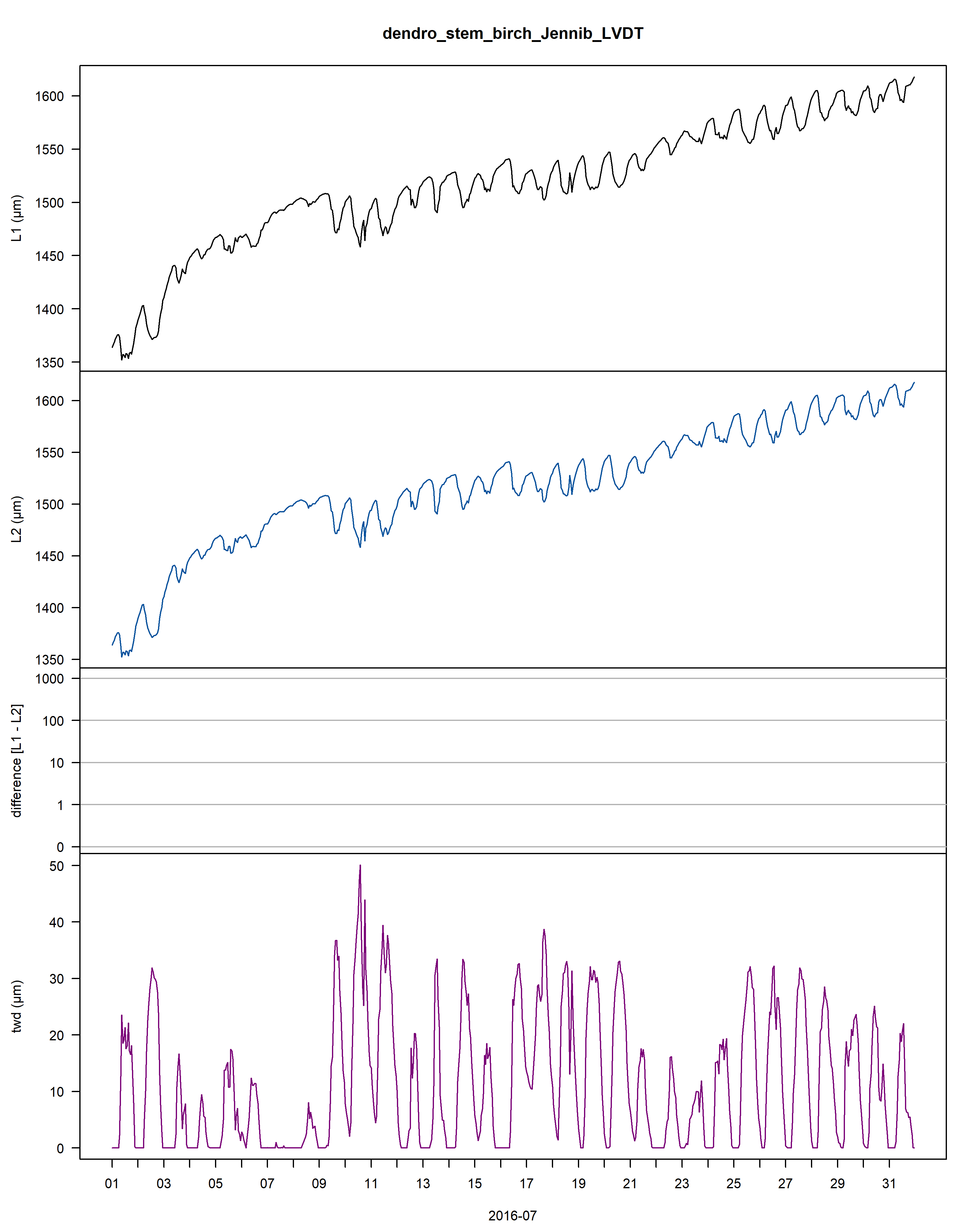
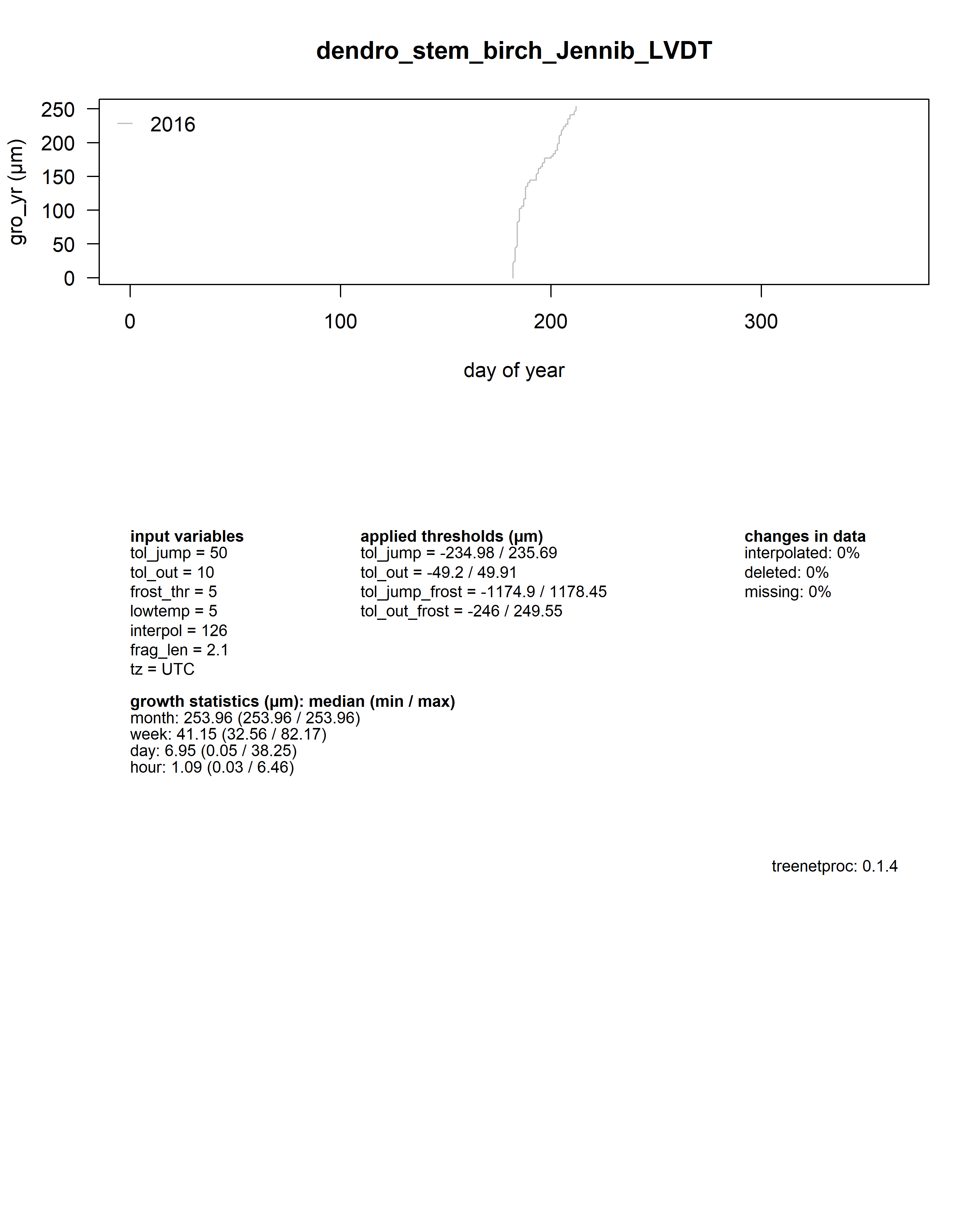
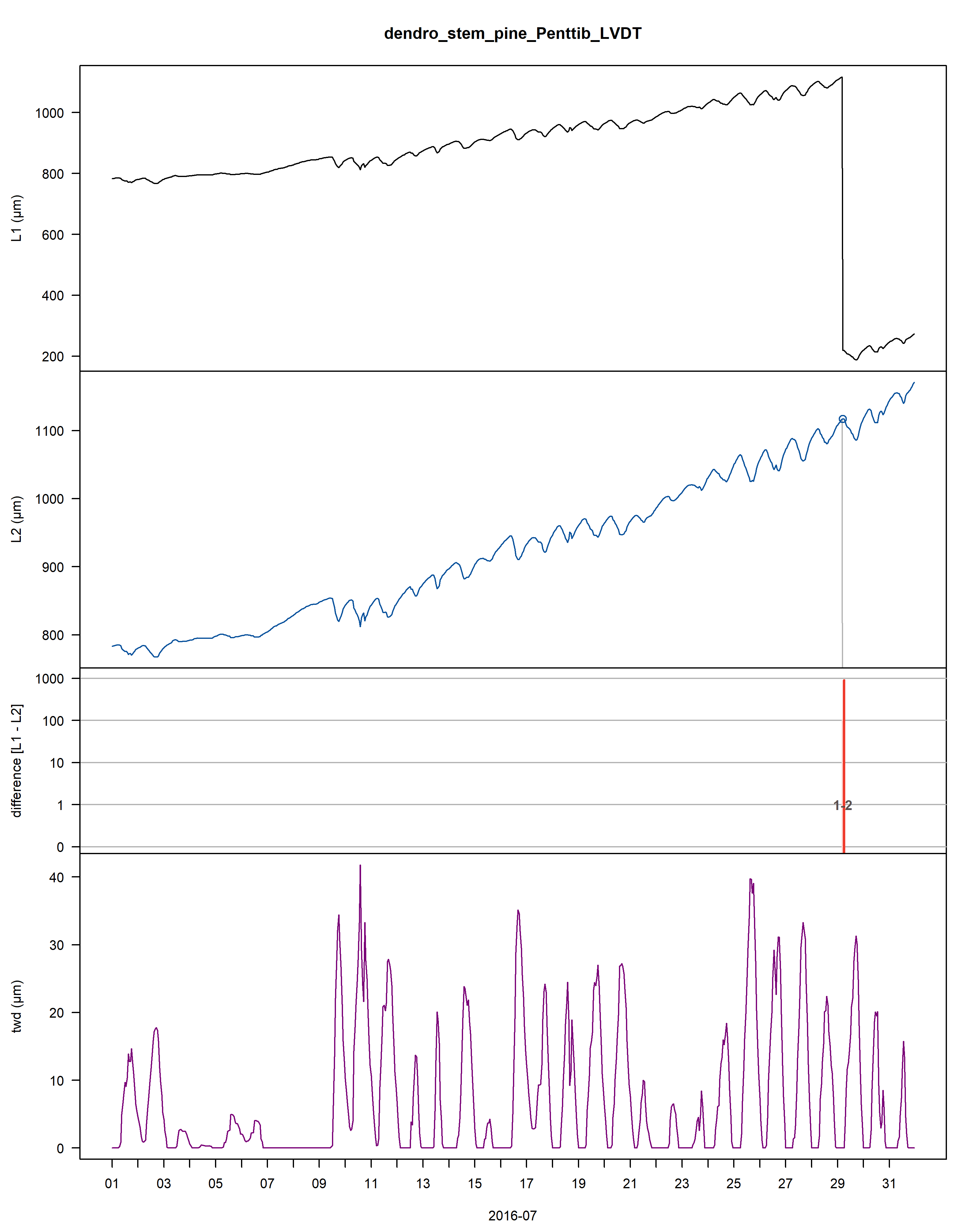
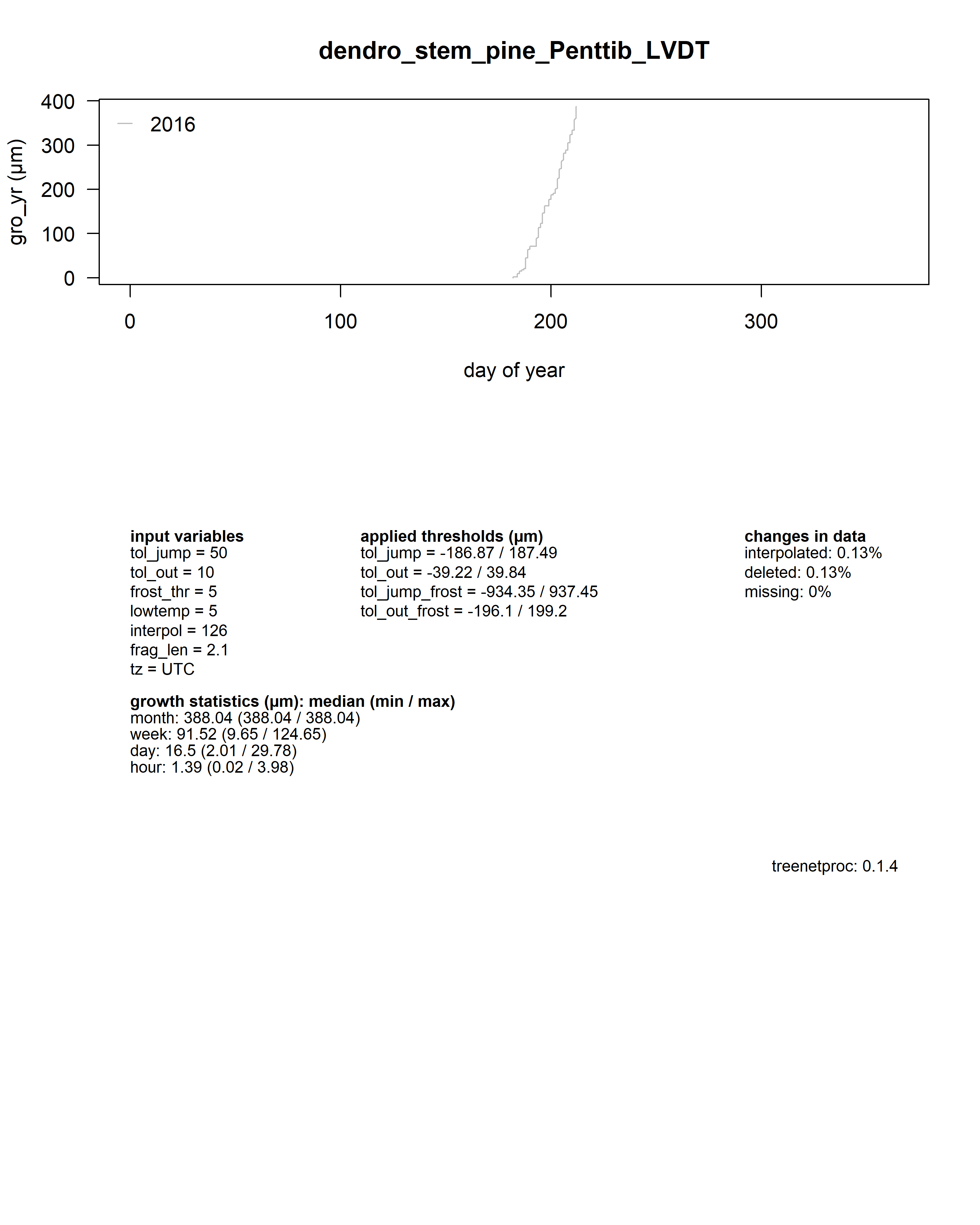
Figure: The plot contains an example of the data, with 1) the stem radius changes of the raw time-aligned L1 dendrometer data in the first panel, 2) the stem radius changes of the cleaned L2 dendrometer data (with L1 data in the background in grey) in the second panel. Interpolated points are circled and frost periods are indicated with a horizontal, cyan line, 3) the changes between L1 and L2 data (red) as well as the deleted values (pink) in the third panel, 4) and the tree water deficit (twd) in the last panel.
As a summary for each dendrometer series, an additional plot shows the yearly growth curves aligned by the day of year.
Beneath the plot all input values, some growth statistics as well as the package version used are reported.
When scrolling through to July 2009 (2009-07), one can see that although most of the errors (induced by sensor failure) have been removed some manual removing is still required. For more examples on using treenetproc, use this link: https://deep-tools.netlify.app/2020/11/21/treenetproc-intro/
6. Data Interpretation
Assignment
The processed dendrometer data provides information on the amount of growth (column gro_yr in dendro_data_L2). From the pdf files it is clear that the growing season of these trees runs from April till August. These months can be isolated by using the ts column and one could then assess for both tree species how much growth was obtained in each year (difference between the minimum gro_yr and maximum gro-yr). An example on how to isolate these specific months is provided below:
# isolate a tree species and the growth data (column 6)
sel<-as.data.frame(dendro_data_L2)
input<-sel[which(sel$series=="dendro_stem_birch_Jennib_LVDT"),c(2,6)]

# add years and months as seperate columns
input$month<-as.factor(right(left(input$ts,7),2))
input$years<-as.factor(left(input$ts,4))

# isolating values within the growing season
input<- input[which(as.character(input$month)%in%c("04","05","06","07","08","09")),]

# calculating the minimum and maximum values per year
minimum_input<-aggregate(input$gro_yr,by=list(input$years),min,na.rm=T)
maximum_input<-aggregate(input$gro_yr,by=list(input$years),max,na.rm=T)

# the difference between the minimum and maximum gro_yr represents the growth in micrometers
head(data.frame(year=maximum_input$Group.1,growth_micron=maximum_input$x-minimum_input$x))
##   year growth_micron
## 1 2015      646.4647
## 2 2016      846.4683
## 3 2017      960.7054
## 4 2018      504.8890
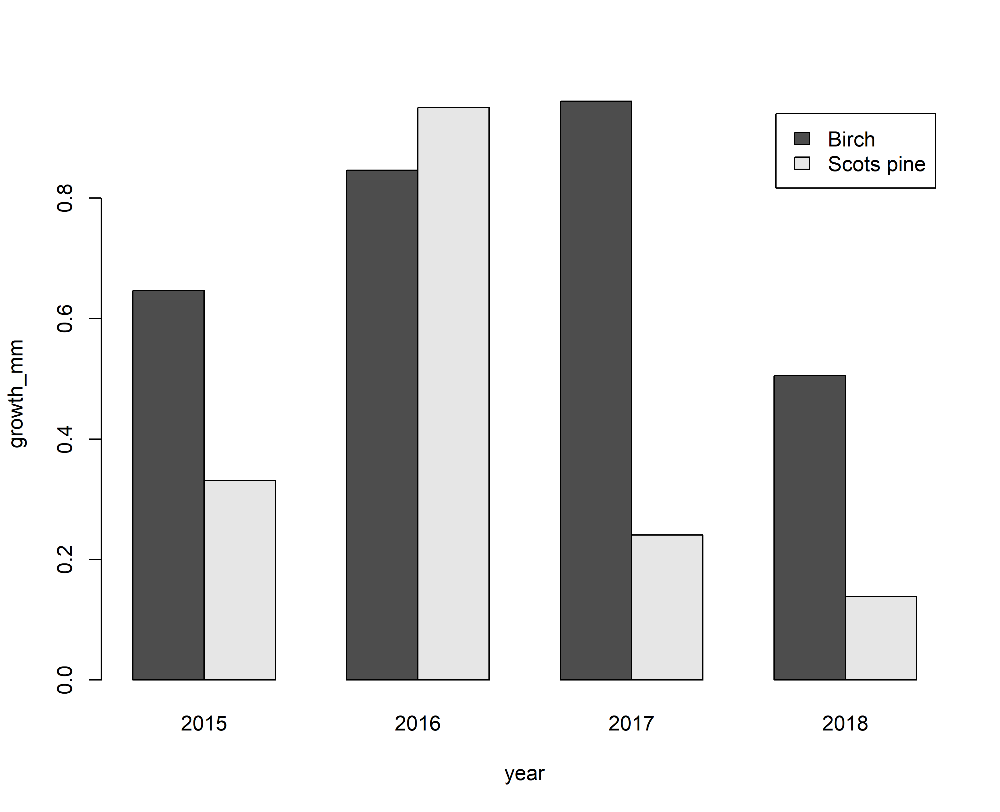
With this example in mind, one can produce a plot showing the annual growth rates per year and tree. Produce such a graph and answer the following questions:
-
- Which tree showed the higher growth rate and by how much?
-
- Which year was an exceptionally good growth year for either tree?
#ANSWER FOR PARTICIPANTS [hidden in provided version]
# prepare the data for birch
sel<-as.data.frame(dendro_data_L2)
input<-sel[which(sel$series=="dendro_stem_birch_Jennib_LVDT"),c(2,6)]
input$month<-as.factor(right(left(input$ts,7),2))
input$years<-as.factor(left(input$ts,4))
input<- input[which(as.character(input$month)%in%c("04","05","06","07","08","09")),]
minimum_input<-aggregate(input$gro_yr,by=list(input$years),min,na.rm=T)
maximum_input<-aggregate(input$gro_yr,by=list(input$years),max,na.rm=T)
birch<-data.frame(year=maximum_input$Group.1,growth_micron=maximum_input$x-minimum_input$x)
birch$tree<-"Birch"

# prepare the data for pine
sel<-as.data.frame(dendro_data_L2)
input<-sel[which(sel$series=="dendro_stem_pine_Penttib_LVDT"),c(2,6)]
input$month<-as.factor(right(left(input$ts,7),2))
input$years<-as.factor(left(input$ts,4))
input<- input[which(as.character(input$month)%in%c("04","05","06","07","08","09")),]
minimum_input<-aggregate(input$gro_yr,by=list(input$years),min,na.rm=T)
maximum_input<-aggregate(input$gro_yr,by=list(input$years),max,na.rm=T)
pine<-data.frame(year=maximum_input$Group.1,growth_micron=maximum_input$x-minimum_input$x)
pine$tree<-"Scots pine"

# merge data together (convert to mm)
input<-rbind(birch,pine)
input$tree<-as.factor(input$tree)
input$growth_mm<-input$growth_micron*0.001
barplot(growth_mm~tree+year,data=input,beside=T,legend=T)
# maximum growth rates per species
max_growth<-aggregate(input$growth_mm,by=list(input$tree),max,na.rm=T)
diff(max_growth$x)
## [1] -0.01043714

# Question 1: Birch growth faster with a maximum value of 0.01 mm.
# Question 2: Birch grows faster in 2017, while Scots pine grows better in 2016.
Assignment
Tree water deficit (column twd) has also been calculated. TWD provides information on how much the tree has shrunk and thus provides information on the water stress a tree experienced during specific periods. Although the site is relatively wet and cold, some summer months can cause measurable water loss for these individuals. During the peak summer month (July) water loss can be quite substantial. Using this TWD information one could ask:
-
- Which tree showed more shrinkage during the peak summer month?
-
- Which year was more water demanding? To answer these question please generate a bloxplot illustrating the TWD statistics during the peak summer month.
#ANSWER FOR PARTICIPANTS [hidden in provided version]
# prepare the data for birch
sel<-as.data.frame(dendro_data_L2)
input<-sel[which(sel$series=="dendro_stem_birch_Jennib_LVDT"),c(2,5)]
input$month<-as.factor(right(left(input$ts,7),2))
input$years<-as.factor(left(input$ts,4))
input<- input[which(as.character(input$month)%in%c("07")),]
birch<-data.frame(year=input$years,twd=input$twd)
birch$tree<-"Birch"

# prepare the data for pine
sel<-as.data.frame(dendro_data_L2)
input<-sel[which(sel$series=="dendro_stem_pine_Penttib_LVDT"),c(2,5)]
input$month<-as.factor(right(left(input$ts,7),2))
input$years<-as.factor(left(input$ts,4))
input<- input[which(as.character(input$month)%in%c("07")),]
pine<-data.frame(year=input$years,twd=input$twd)
pine$tree<-"Scots pine"

# merge data together (convert to mm)
input<-rbind(birch,pine)
input$tree<-as.factor(input$tree)
input$twd_mm<-input$twd*0.001
boxplot(twd_mm~tree+year,data=input,col=c("grey90","grey40"))
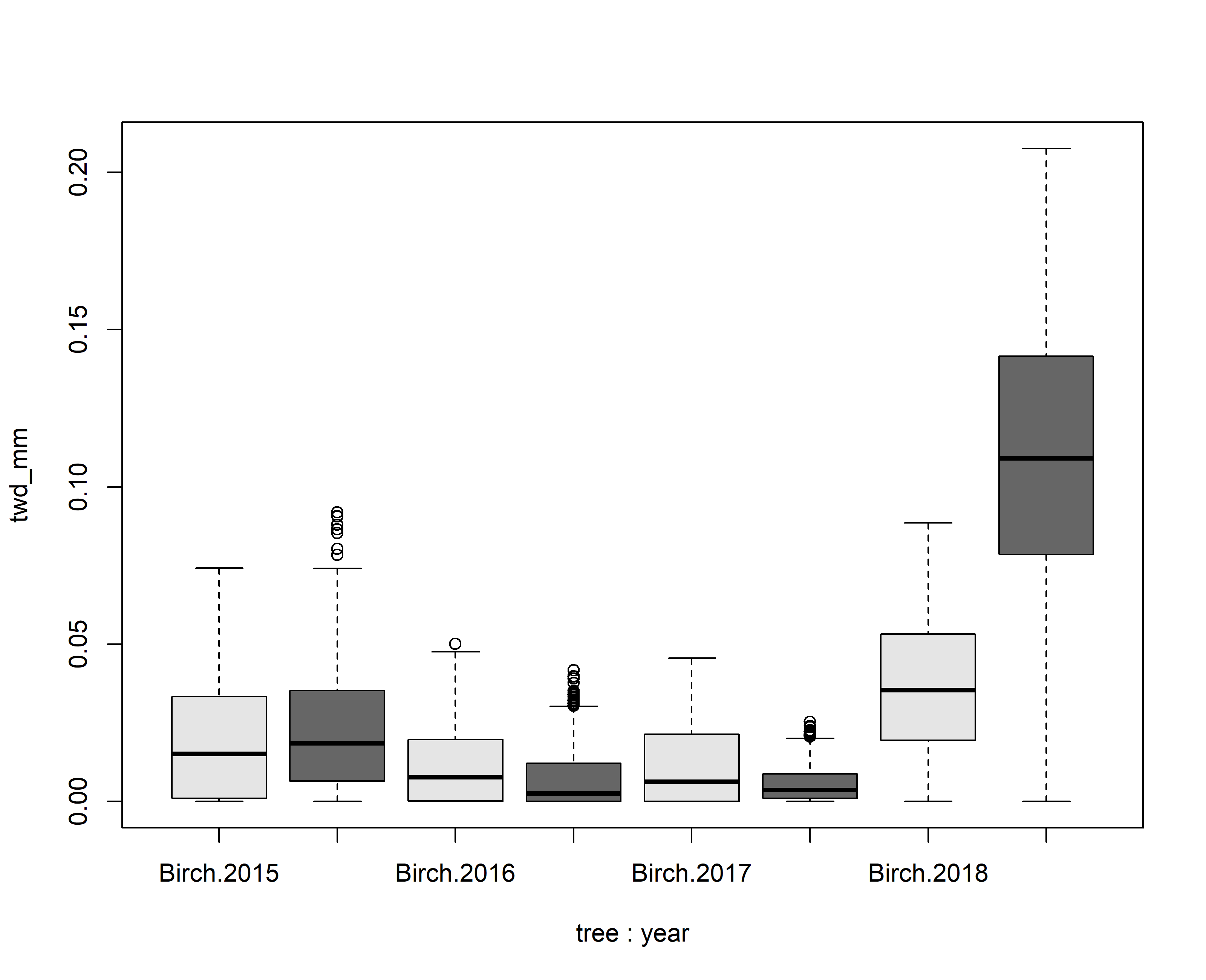
# Question 1: Scots pine showed more shrinkage.
# Question 2: For both species 2018 was the year with the most severe shrinkage.
7. Using treeprocnet
For use in publication, the reference is:
citation("treenetproc")
##
## To cite treenetproc in publications use:
##
##   Knüsel S., Haeni M., Wilhelm M., Peters R.L., Zweifel R. 2020.
##   treenetproc: towards a standardized processing of stem radius data.
##   In prep.
##
##   Haeni M., Knüsel S., Wilhelm M., Peters R.L., Zweifel R. 2020.
##   treenetproc - Clean, process and visualise dendrometer data. R
##   package version 0.1.4. Github repository:
##   https://github.com/treenet/treenetproc
##
##   Hadley Wickham, Romain François, Lionel Henry and Kirill Müller
##   (2019). dplyr: A Grammar of Data Manipulation. R package version
##   0.8.3. https://CRAN.R-project.org/package=dplyr
##
## To see these entries in BibTeX format, use 'print(<citation>,
## bibtex=TRUE)', 'toBibtex(.)', or set
## 'options(citation.bibtex.max=999)'.
8. References
- Pappas C, Peters RL, Fonti P (2020) Linking variability of tree water use and growth with species resilience to environmental changes. Ecography. 43: 1-14.
- Knüsel S, Haeni M, Wilhelm M, Peters RL, Zweifel R (2020) treenetproc: towards a standardized processing of stem radius data. In prep.
- Zweifel R, Haeni M, Buchmann N, Eugster W (2016) Are trees able to grow in periods of stem shrinkage? New Phytol. 211:839-49.
See also:
9. Contact
For questions, please get in touch with Richard Peters