RAPTOR Workflow

1. Background

The package RAPTOR performs wood cell anatomical data analyses on spatially explicit xylem (tracheids) data sets derived from wood anatomical thin sections. The package includes functions for the visualization, alignment and detection of continuous tracheid radial file (defines as rows) and tracheid position within an annual ring of coniferous species. This tutorial presents and example for generating tracheidograms for a Pinus sylvestris, yet the package include example for Picea abies, Pinus cembra and Pinus sylvestris.

2. Set-up steps

#install package if necessary
packages <- (c("RAPTOR","tgram"))
install.packages(setdiff(packages, rownames(installed.packages())))
library(RAPTOR)
library("tgram")
## Loading required package: zoo
## 
## Attaching package: 'zoo'
## The following objects are masked from 'package:base':
## 
##     as.Date, as.Date.numeric

The package’s functions are to be executed sequentially:

1. is.raptor(),
2. graph.cells(),
3. align(),
4. first.cell(),
5. pos.det(),
6. write.output(),
7. batch.mode() is a convenient ‘wrapper’ function streamlining steps 1 through 6
8. anatomy.data calls complimentary example data sets.

Each function is complimented by detailed documentation, which can be accessed by calling a function’s name preceded by a question mark.

?is.raptor()
## starting httpd help server ... done

3. Import data

The package uses tracheid anatomical data obtained from quantitative wood anatomy software (e.g., ROXAS, WinCELL, ImageJ), with the specific positional information necessary for the automated construction of tracheidograms. To provide positional output, RAPTOR requires input data to be formatted into an R data-frame object with a designated row for each tracheid, as typically obtained from measurements performed on images of thin cross-sections of wood increment cores.

#- examples provided with the package
?anatomy.data

The input data-frame must include six specific columns:

• an identifier column for the wood sample (e.g., ID),
• an identifier for the tracheid (e.g., CID),
• the year of the dated tree ring (e.g., YEAR),
• the cell lumen area (e.g., CA),
• and the x- and y-coordinates of the centroid of the tracheid lumen (e.g., XCAL and YCAL).

Commonly used software’s provide the information on CID, CA (in ROXAS LA, which needs to be transformed), XCAL and YCAL, while the ID and YEAR can be added afterwards. These column names must either match the names mentioned above or columns have to be ordered according to the order presented here.

# included example datasets
as.character(unique(anatomy.data[,"ID"]))
## [1] "LOT_PICEA"   "LOW_PINUS"   "SIB_LARIX"   "MOUNT_PINUS"

For this example we will use the Scots pine (Pinus sylvestris) example from the Eastern lowlands in Germany (named: “LOW_PINUS”), collected using the ROXAS software.

# validating example data
input_raw<-example.data(species="LOW_PINUS")

# temporal range of the dataset
unique(input_raw[,"YEAR"])
## [1] 2007 2008 2009 2010

The dataset includes 4 years, ranging from 2007 until 2010.

# general statistics of the dataset
summary(input_raw)
##            ID            CID            YEAR            CA         
##  LOT_PICEA  :   0   Min.   :7949   Min.   :2007   Min.   :   2.04  
##  LOW_PINUS  :2011   1st Qu.:8452   1st Qu.:2008   1st Qu.: 216.06  
##  MOUNT_PINUS:   0   Median :8954   Median :2008   Median : 434.11  
##  SIB_LARIX  :   0   Mean   :8954   Mean   :2008   Mean   : 504.34  
##                     3rd Qu.:9456   3rd Qu.:2009   3rd Qu.: 742.27  
##                     Max.   :9959   Max.   :2010   Max.   :1574.22  
##                                                                    
##       XCAL              YCAL            CWTALL     
##  Min.   :-471.57   Min.   :155827   Min.   :1.590  
##  1st Qu.: -81.62   1st Qu.:157677   1st Qu.:3.690  
##  Median : 117.56   Median :159157   Median :4.610  
##  Mean   : 177.00   Mean   :159072   Mean   :4.743  
##  3rd Qu.: 380.29   3rd Qu.:160526   3rd Qu.:5.758  
##  Max.   :1005.65   Max.   :161853   Max.   :8.340  
##                                     NA's   :5

The data illustrates that the lumen area is on average 504 square micron, while mean cell wall thickness is 4.7 micron.

# mean properties per year
stats::aggregate(input_raw[,c(4,7)],by=list(input_raw$YEAR),mean,na.rm=T)
##   Group.1       CA   CWTALL
## 1    2007 402.2410 5.159179
## 2    2008 533.1832 4.710089
## 3    2009 517.0780 4.584225
## 4    2010 588.9568 4.417276

This table illustrates that cell wall thickness (CWTALL) is slowly decreasing, while lumen area (or cell area, CA) is increasing.

4. Data verification and visualization

The user can verify if a data-frame fits the requirements for RAPTOR data format by using the function is.raptor().

# input validation
?is.raptor
data<-is.raptor(input_raw,str=TRUE)
## 'data.frame':	2011 obs. of  7 variables:
##  $ ID    : Factor w/ 4 levels "LOT_PICEA","LOW_PINUS",..: 2 2 2 2 2 2 2 2 2 2 ...
##  $ CID   : int  7949 7950 7951 7952 7953 7954 7955 7956 7957 7958 ...
##  $ YEAR  : int  2007 2007 2007 2007 2007 2007 2007 2007 2007 2007 ...
##  $ CA    : num  494 756 376 406 1063 ...
##  $ XCAL  : num  -165 -220 -247 -160 -268 ...
##  $ YCAL  : num  155827 155841 155850 155859 155875 ...
##  $ CWTALL: num  4.23 3.73 2.8 3.07 3.39 3.09 3.4 3 3.38 3.19 ...
## NULL

Here the structure of the RAPTOR file is printed.

# plottng data for 2009
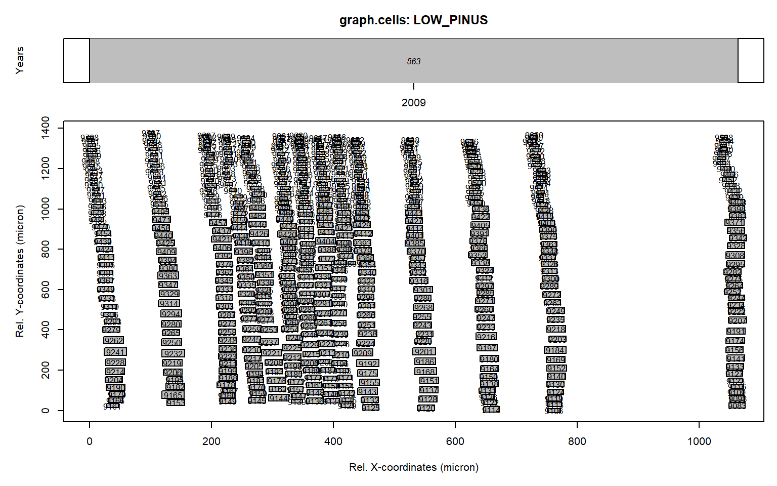
graph.cells(data,year=2009)

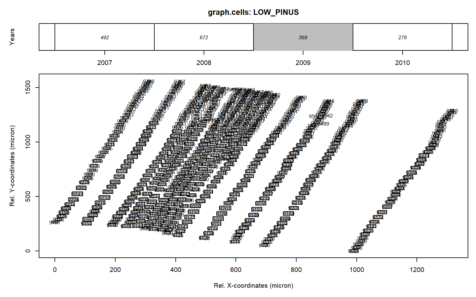
Figure 1: Graphical representation of anatomical data presented with the function graph.cells() for the ring 2007 from the LOW_PINUS example. The upper panel indicates the calendar year for each ring and its total number of cells. The lower panel provides the positional data and the lumen area of each tracheid (size of the square) for the grey coloured annual ring shown in the upper panel. When plotting in R the number within the rectangle provides the cell identifier.

One can also plot the data interactively by using interact = TRUE as an additional argument in graph.cells(). The numbers within the grey cells indicate the CID provided wtihin RAPTOR file, which shows that CID 9317, 9499, 9542, 9557 and 9679 are cell not part of a potential full row.

outliers<-data[which(data$CID%in%c(9517, 9499, 9542, 9537,9679)),]
par(mfrow=c(1,1))
par(mar=rep(5,4))
data.2009<-data[which(data$YEAR==2009),]
plot(data.2009$XCAL,data.2009$YCAL,pch=16,ylab="YCAL",xlab="XCAL")
points(outliers$XCAL,outliers$YCAL,col="orange",pch=16)
legend("topleft",c("Cells","Outliers"),pch=16,col=c("black","orange"),bty="n")

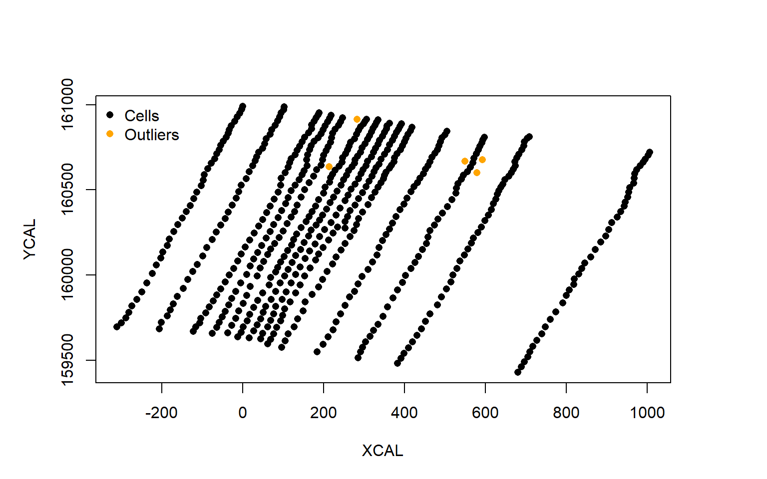
First on can see that the X- and Y-axis are scaled to the minimum values within graph.cells(). Second the orange cells indeed appear to be outliers and can to be removed to improve the row detection.

# manually remove outliers
data<-data[which(data$CID%in%c(9517, 9499, 9542, 9537,9679)==F),]
graph.cells(data,year=2009)

As this manual editing is quite labor intensive we created an interactive cleaning tool called datacleanr.

5. Main RAPTOR functionalities

When running the functions to detect the first cells and row in which the individual cell belong to one is confronted with rotational issues.

# default identification of rows
data.2009<-data[which(data$YEAR==2009),]
first<-first.cell(data.2009, frac.small = 0.2, yrs = FALSE, make.plot = FALSE)
pos.det(first, swe = 0.7, sle = 3, ec = 1.75, swl = 0.5, sll = 5, lc = 10,
        prof.co = 1.7, max.cells = 0.7, yrs = FALSE, aligning = FALSE, make.plot = TRUE)

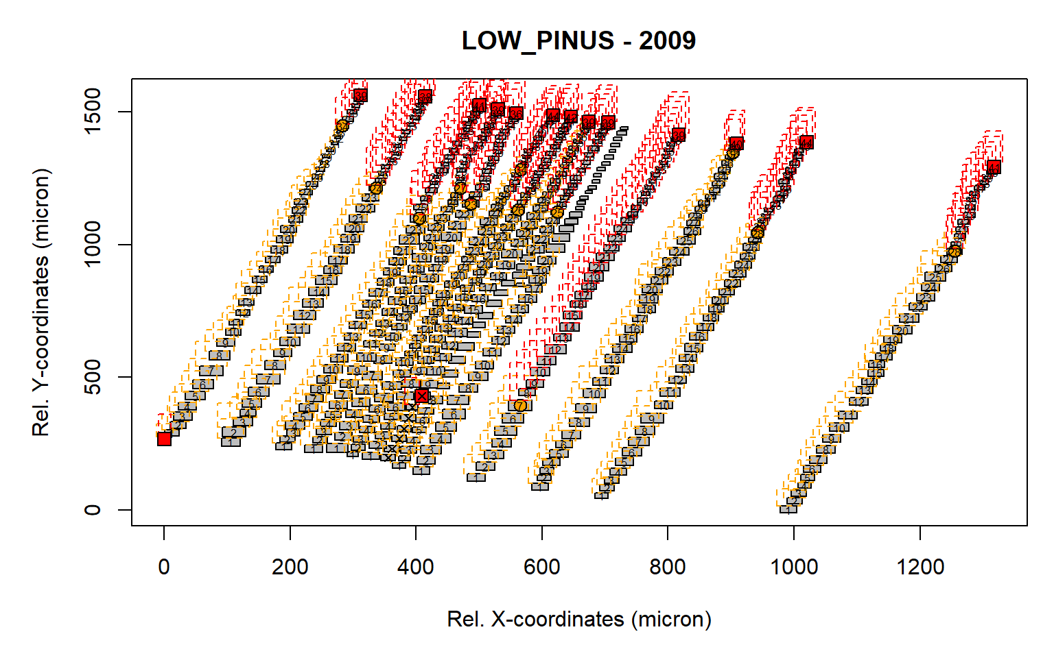
Figure 2: Visual representation of the identified rows. A similar graph is presented as the graph.cells() function. The orange boxes illustrate the search area for the earlywood cells (defined by "swe = 0.7" and "sle = 3"), while the red boxes indicate the search the search area for the latewood cells (defined by "swl = 0.5" and "sll = 5"). The orange dot indicates the end of the earlywood search, while the red square indicates the end of the latewood search.Numbers within the gray cells indicate CID which are assigned to a row.

##              ID  CID YEAR      CA    XCAL    YCAL CWTALL ROW POSITION MARKER
## 12820 LOW_PINUS 9083 2009  693.15  991.40    1.00   3.15  13        1     NA
## 12835 LOW_PINUS 9098 2009  602.57 1000.79   33.95   2.78  13        2     NA
## 12843 LOW_PINUS 9106 2009  444.33  694.57   54.48   5.04  12        1     NA
## 12846 LOW_PINUS 9109 2009  555.12 1007.52   63.37   3.07  13        3     NA
## 12850 LOW_PINUS 9113 2009  533.74  703.48   84.20   7.21  12        2     NA
## 12851 LOW_PINUS 9114 2009  667.74  597.01   87.09   3.99  11        1     NA
## 12853 LOW_PINUS 9116 2009  420.55 1016.34   91.97   3.28  13        4     NA
## 12856 LOW_PINUS 9119 2009  547.93  710.50  112.37   5.15  12        3     NA
## 12857 LOW_PINUS 9120 2009  802.06  495.31  122.30   4.10  10        1     NA
....

It is clear that some of the rows are not correctly detected due to the rotation of the sample (as some boxes are not filled with numbers). A rotation of the sample is thus required to improve the row detection.

# automatic rotation of the sample rotation of sample
align(data.2009,make.plot=TRUE)

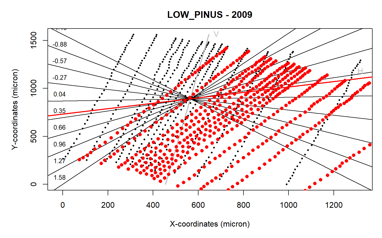
Figure 3: Tree-ring alignment for the ring 2009 from the LOW_PINUS example. Plot obtained from the align() function where a crosshair is provided to assess the rotational angle (expressed as the slope of a linear regression) required for optimizing the alignment of the radial growth axis of the ring to the image y-axis.

##              ID  CID YEAR      CA       XCAL       YCAL CWTALL
## 12820 LOW_PINUS 9083 2009  693.15  954.40888    0.00000   3.15
## 12835 LOW_PINUS 9098 2009  602.57  972.39472   29.16135   2.78
## 12843 LOW_PINUS 9106 2009  444.33  683.25996  132.08490   5.04
## 12846 LOW_PINUS 9109 2009  555.12  986.86184   55.64779   3.07
## 12850 LOW_PINUS 9113 2009  533.74  699.90662  158.26801   7.21
## 12851 LOW_PINUS 9114 2009  667.74  598.22328  189.96520   3.99
## 12853 LOW_PINUS 9116 2009  420.55 1003.11770   80.77744   3.28
## 12856 LOW_PINUS 9119 2009  547.93  714.31335  183.47268   5.15
## 12857 LOW_PINUS 9120 2009  802.06  509.90833  251.47213   4.10
....

The automated detection does not appear to work as the sample is rotated in the wrong direction (red dots vs the original black dots).

# interactive rotation of the sample rotation of sample
align<-align(data.2009,interact=TRUE)
-0.27
y

The interactive rotation generates a similar figure where one can select the line which best described the radial alignment of the cells (linear slope: -0.27).

# plotting aligned data
graph.cells(align)

This new figure (originating from the graph.cells() function) illustrates that the rotation was correct (all rows of tracheids are aligned vertically).

The next step is to detect the first cell of each tracheidogram.

#- first cell detection
?first.cell
first<-first.cell(align, make.plot=TRUE, frac.small=0.5)

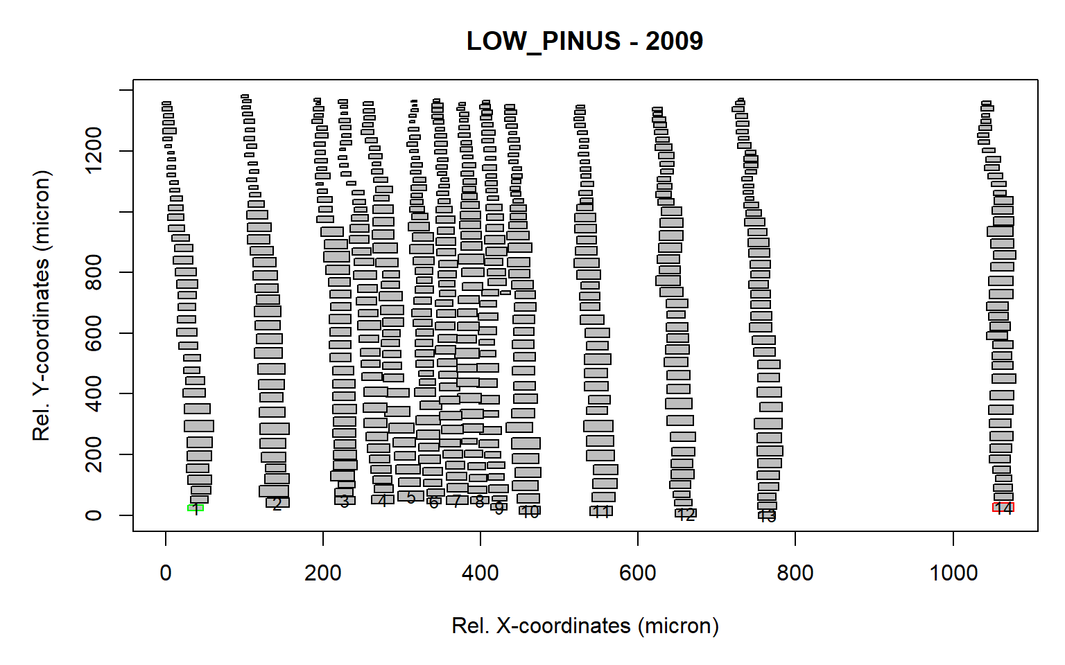
Figure 4: Tree ring after the rotation and identification of the first cells (as a result of the first.cell() function). The first and last identified cells are marked in green and red respectively. A total of 14 first cells (indicated with numbers) were detected.

The frac.small=0.5 is a numeric value (between 0 and 1) that is multiplied by the average cell lumen size of the ring, determining the minimum threshold used to exclude cells in the first row that are too small. This is useful when latewood cells from the previous ring are present within the sample.

Next, the recognition of continuous radial files ??? i.e., radial files which display an uninterrupted sequence of cells from the start to the end of the ring ??? and the assignment of a tracheid cell’s position within each radial file, is obtained using the function pos.det(). Before running this function one should carefully study the multitude of parameters that are included within this function.

# parameter overview for detecting radial files (or cell rows)
?pos.det

By looping through each identified first-row cell, this function uses another algorithm to identify the next sequential tracheid in the radial file. The algorithm is instructed by user-defined “earlywood” and “latewood” variables, dependent on the anatomical characteristics of the wood sample (cf. package description). The algorithm moves from one target cell (n), to the next (n + 1) using a rectangular search grid. The width and the length of the grid are defined as the proportion of a target cell’s lumen diameter (where Ln = CAn1/2) multiplied by sle (sl = search length) and swe (sw = search width) for larger earlywood cells (e) and sll and swl for smaller latewood cells (l). If more than one tracheid falls within the rectangular search grid, the closest tracheid will be selected. Specified size ratio variables between consecutive tracheid (i.e., ec = earlywood cut off, and lc = latewood cut off) are used to stop the algorithm search when unrealistically small cells are detected. Finally, the arguments prof.co (i.e., a threshold ratio of distance to the previous [between n and n-1] and the consecutive tracheid [n and n + 1]), and max.cell (expressed as a proportion of the annual maximum number of radial file cells) can be used to filter out incomplete radial files.

# determining the cell position
det.issue<-pos.det(first, swe = 0.7, sle = 3, ec = 1.75, swl = 0.5, sll = 1, lc = 10,
                   prof.co = 1.7, max.cells = 0.7, yrs = FALSE, aligning = FALSE, make.plot = TRUE)

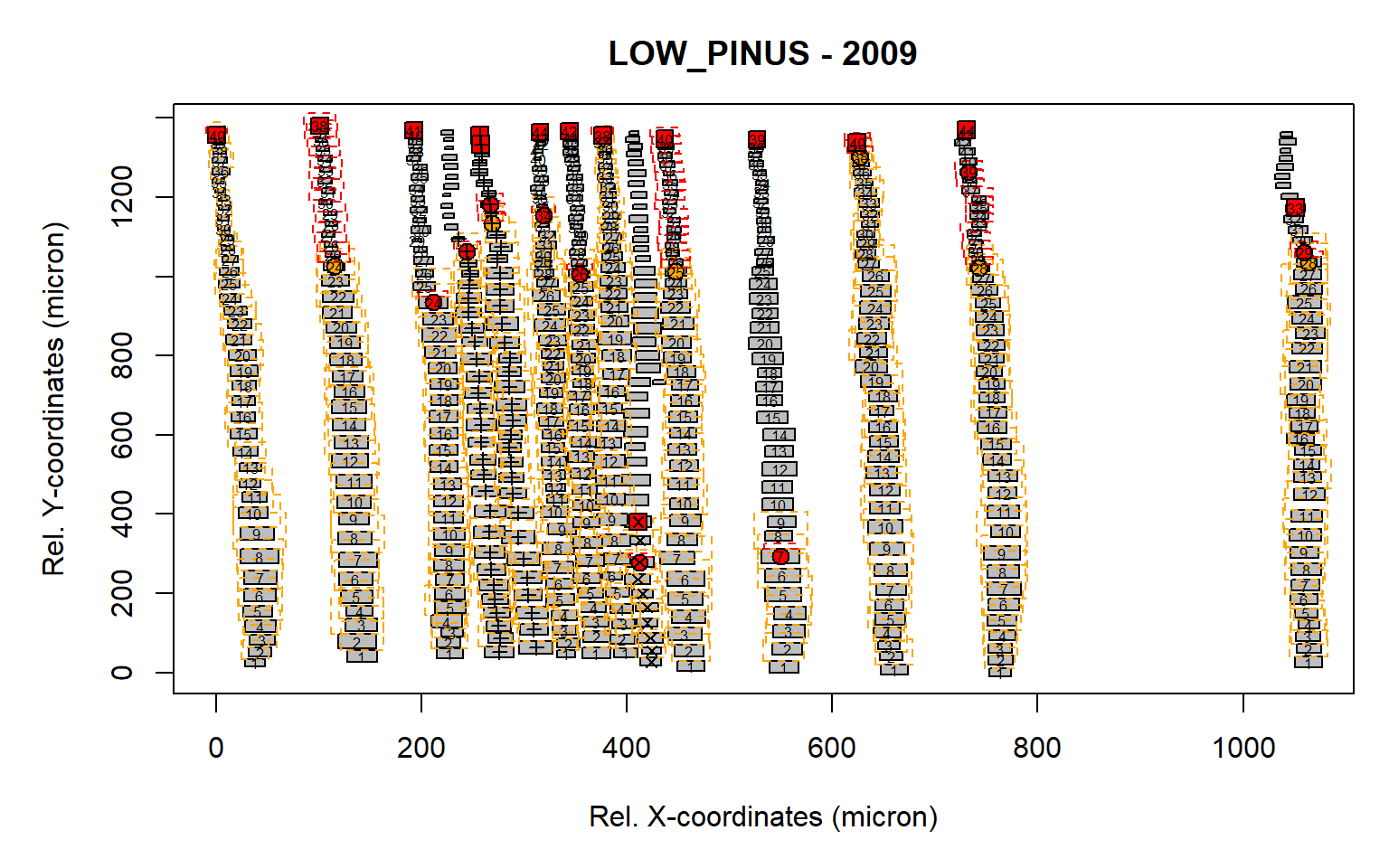
Figure 5: Standard output from the pos.det() function. Here a short latewood search window is selected of 1 (sll).

From this example it is clear that some of the latwood cells have not been detected due to a likely to low search length for the latewood (red boxe, see “sll=1”). As such we need to increase this search length window to 5 (“sll=5”).

# rerun the function
det<-pos.det(first, swe = 0.7, sle = 3, ec = 1.75, swl = 0.5, sll = 5, lc = 10,
             prof.co = 1.7, max.cells = 0.7, yrs = FALSE, aligning = FALSE, make.plot = TRUE)

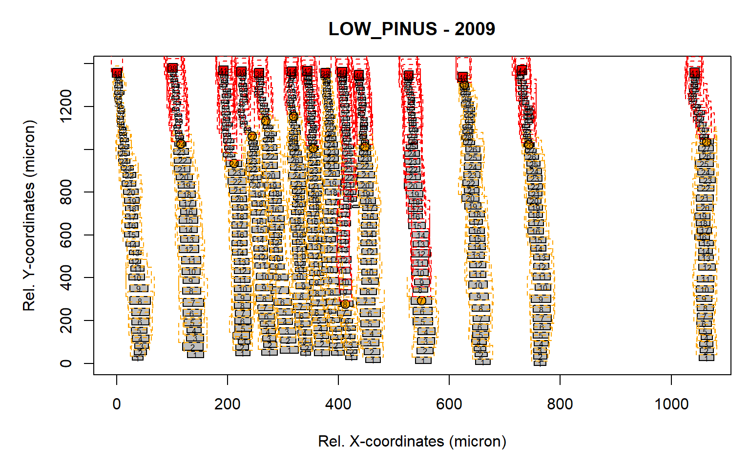
Figure 6: Standard output from the pos.det() function with a larger sll parameter.

The radial file detection seems appropriate as all aligned cells appeared to be assigned to a specific row, where the number indicate the cell number relative to the first cell within the radial file. When satisfied with the results, an ouput file can be generated.

The function write.output() allows the user to export results in numerical (as *.txt) and graphical (as *.pdf) formats to a repository or folder selected by the user.

# generate output
output<-write.output(det)
head(output)

The output file contains the “ROW” and “POSITION” column, with NA’s assigned to tracheids that do not belong to continuous radial files, and a column “MARKER” that tracks RAPTOR decisions in each radial file. Specifically, values are assigned to the last detected “earlywood” cell (value = 1), the last detected “latewood” cell (value = 2), the last detected cell (value = 3), and radial files removed due to gaps (value = 4) or too few cells (value = 5). The function write.output() allows the user to export results in numerical (as *.txt) and graphical (as *.pdf) formats to a repository or folder selected by the user.

6. Batch mode workflow for generating tracheidograms

The batch.mode() function allows the user to automatically run the above functions from a target folder populated by previously prepared files with defined settings. With RAPTOR, we offer access to the characterisation of a significantly increased number of radial files, aiding in the development of more robust and versatile intra-annual anatomical parameters. Also, these measurements provide a better appreciation of the large variability of anatomical parameters among radial files, annual rings, and species.

Below we provide an example of running through all example data included within the RAPTOR package, to illustrate a robust workflow.

Here we run the script for three specific years (2007-2010) per species (including Picea abies, Larix decidua, Pinus cembra and Pinus sylvestris, with the latter being described in the previous example)

# process lowland Pinus sylverstris
par(mfrow=c(1,1))
par(oma=c(0,0,0,0))
par(mar=c(5,5,5,5))
input<-is.raptor(example.data(species="LOW_PINUS") , str = FALSE)
aligned<-align(input,list=c("v","v",-0.26,"h"),make.plot = FALSE)
first<-first.cell(aligned, frac.small = 0.2, yrs = FALSE, make.plot = FALSE)
## [1] "No GAM applied due to low number of rows"
output<-pos.det(first, swe = 0.7, sle = 3, ec = 1.75, swl = 0.5, sll = 5, lc = 10,prof.co = 6, max.cells = 0.5, yrs = FALSE, aligning = FALSE, make.plot = FALSE)
LOW_PINUS<-write.output(output)

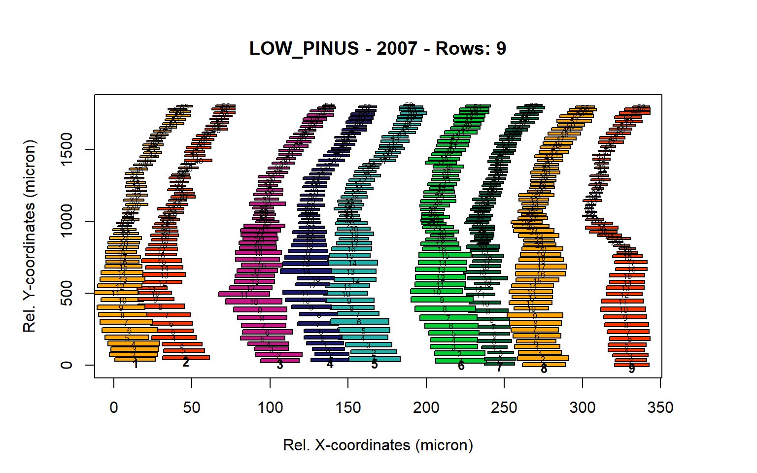
Figure 7: Standard plots generated by the write.output() function for lowland Pinus sylverstris (species="LOW_PINUS"), including 2007, 2008, 2009 and 2010.

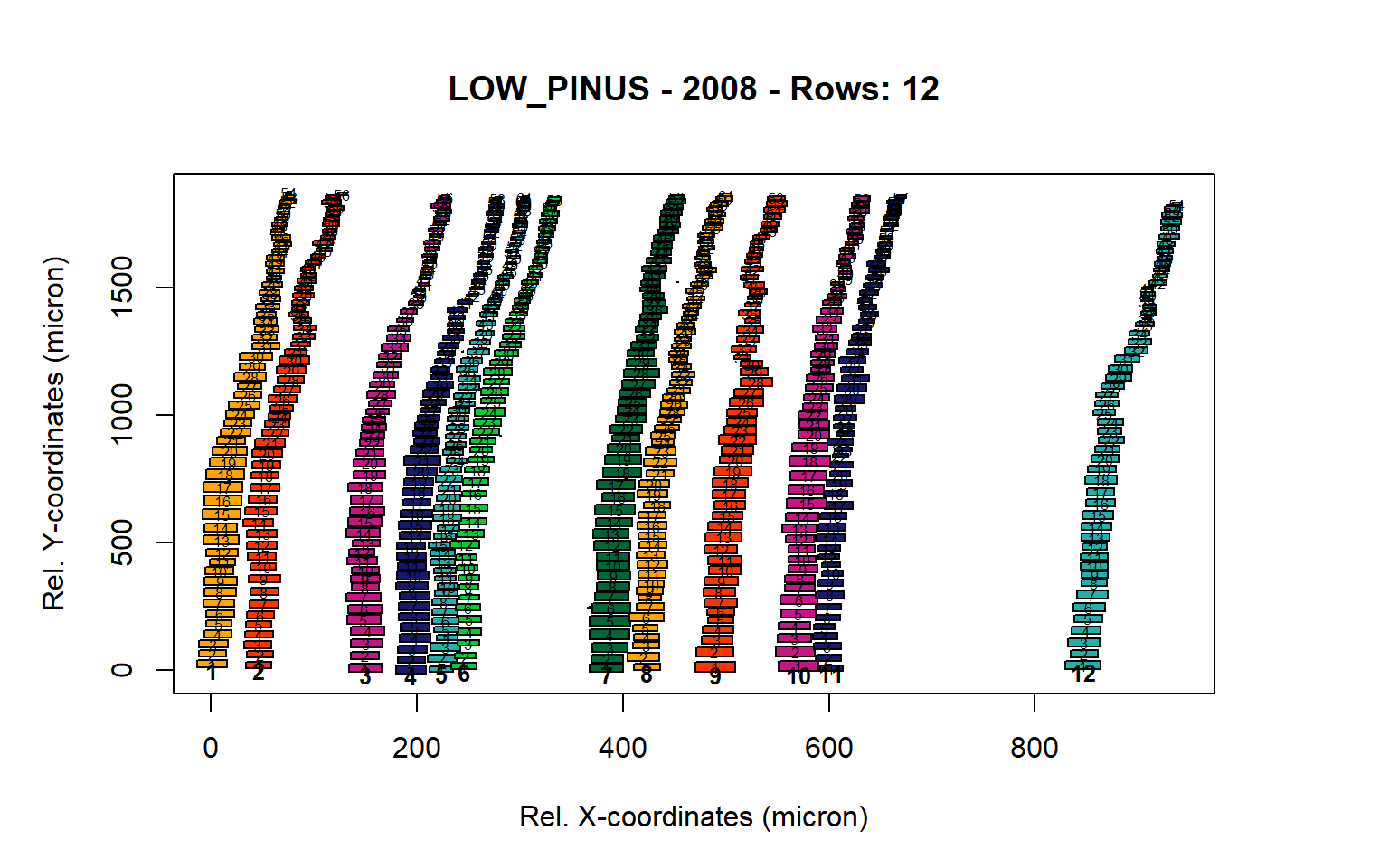
Figure 8: Standard plots generated by the write.output() function for lowland Pinus sylverstris (species="LOW_PINUS"), including 2007, 2008, 2009 and 2010.

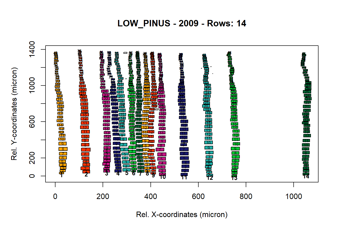
Figure 9: Standard plots generated by the write.output() function for lowland Pinus sylverstris (species="LOW_PINUS"), including 2007, 2008, 2009 and 2010.

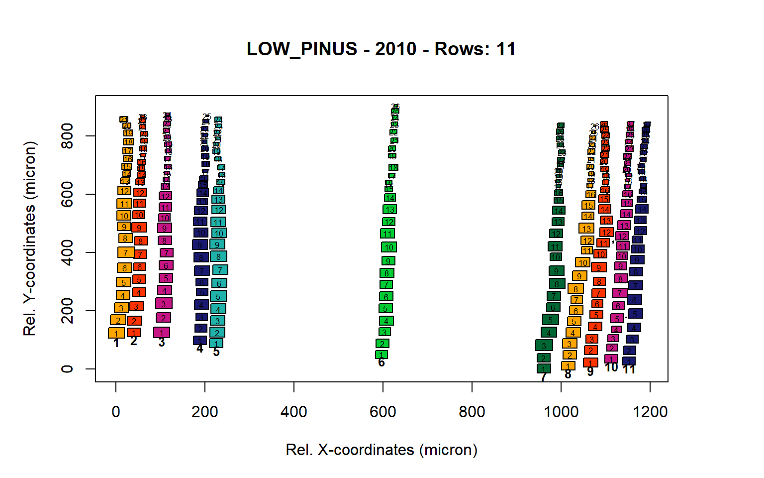
Figure 10: Standard plots generated by the write.output() function for lowland Pinus sylverstris (species="LOW_PINUS"), including 2007, 2008, 2009 and 2010.

# process mountain Pinus cembra
input<-is.raptor(example.data(species="MOUNT_PINUS") , str = FALSE)
aligned<-align(input,list=c("h","h","h",0.03),make.plot = FALSE)
first<-first.cell(aligned, frac.small = 0.2, yrs = FALSE, make.plot = FALSE)
output<-pos.det(first, swe = 0.7, sle = 3, ec = 1.75, swl = 0.5, sll = 5, lc = 10,prof.co = 1.7, max.cells = 0.7, yrs = FALSE, aligning = FALSE, make.plot = FALSE)
MOUNT_PINUS<-write.output(output)

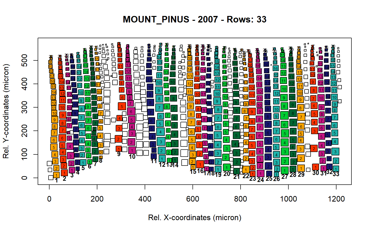
Figure 11: Standard plots generated by the write.output() function for mountain Pinus cembra (species="MOUNT_PINUS"), including 2007, 2008, 2009 and 2010.

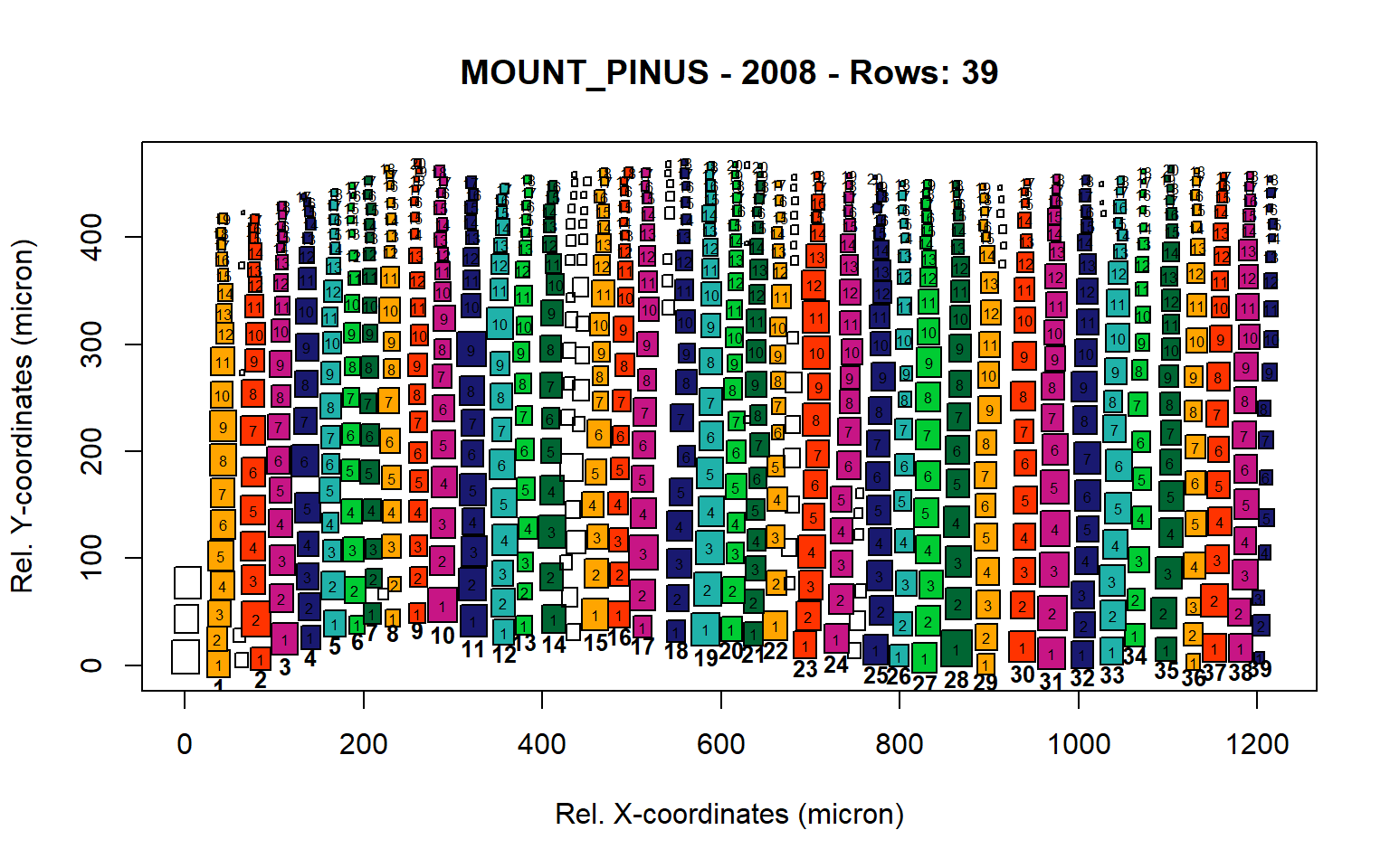
Figure 12: Standard plots generated by the write.output() function for mountain Pinus cembra (species="MOUNT_PINUS"), including 2007, 2008, 2009 and 2010.

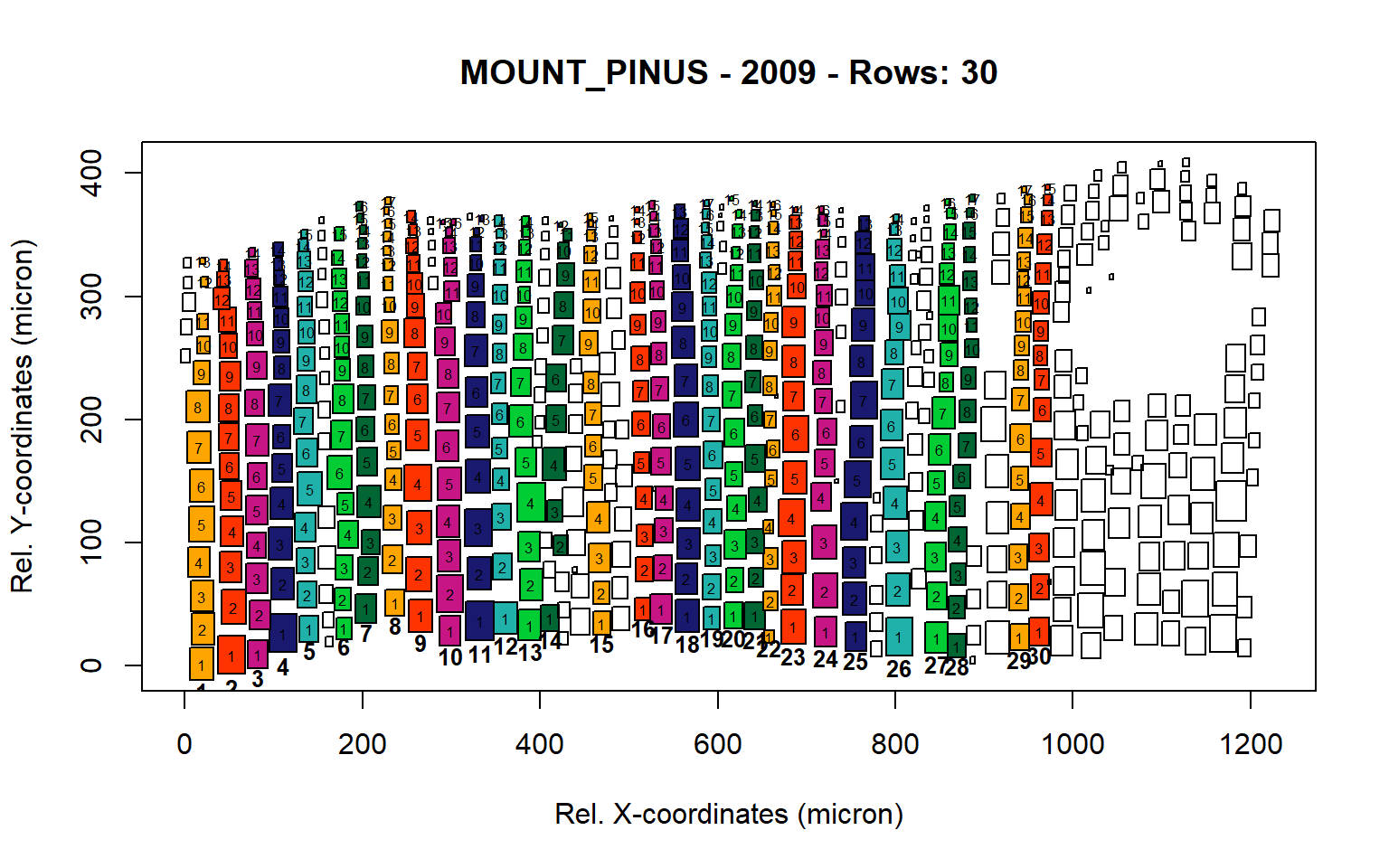
Figure 13: Standard plots generated by the write.output() function for mountain Pinus cembra (species="MOUNT_PINUS"), including 2007, 2008, 2009 and 2010.

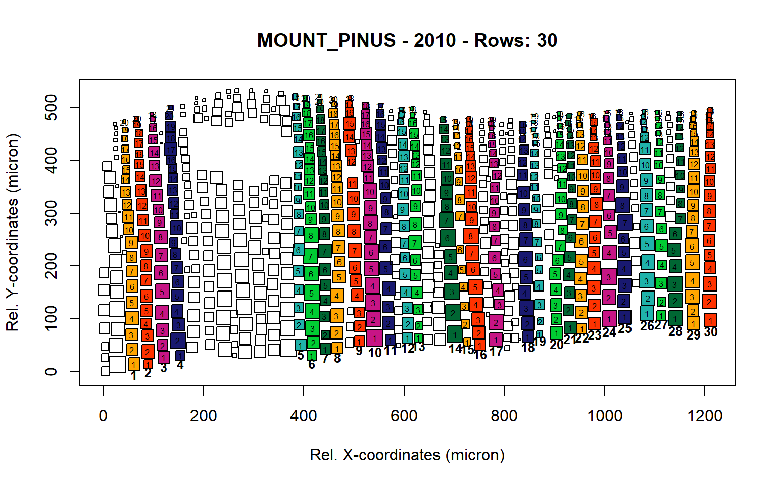
Figure 14: Standard plots generated by the write.output() function for mountain Pinus cembra (species="MOUNT_PINUS"), including 2007, 2008, 2009 and 2010.

# process Siberian Larix siberica

input<-is.raptor(example.data(species="SIB_LARIX") , str = FALSE)
aligned<-align(input)
first<-first.cell(aligned, frac.small = 0.5, yrs = FALSE, make.plot = FALSE)
output<-pos.det(first, swe = 0.3, sle = 3, ec = 1.5, swl = 0.5, sll = 5, lc = 15,prof.co =4, max.cells = 0.5, yrs = FALSE, aligning = FALSE, make.plot = FALSE)
sib_larix<-write.output(output)

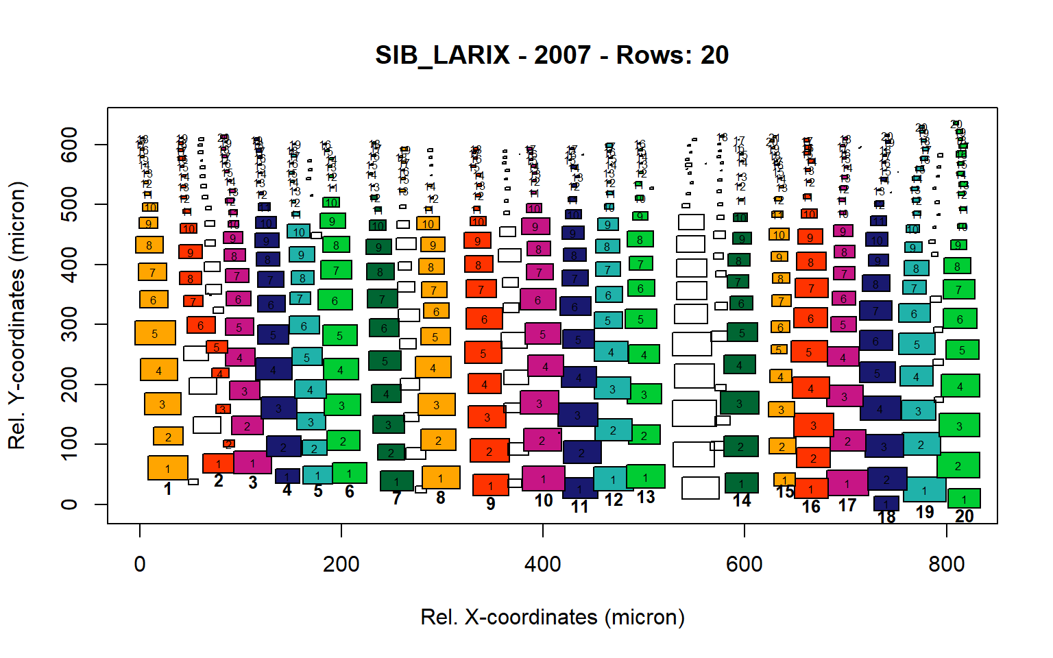
Figure 15: Standard plots generated by the write.output() function for Siberian Larix siberica (species="SIB_LARIX"), including 2007, 2008, 2009 and 2010.

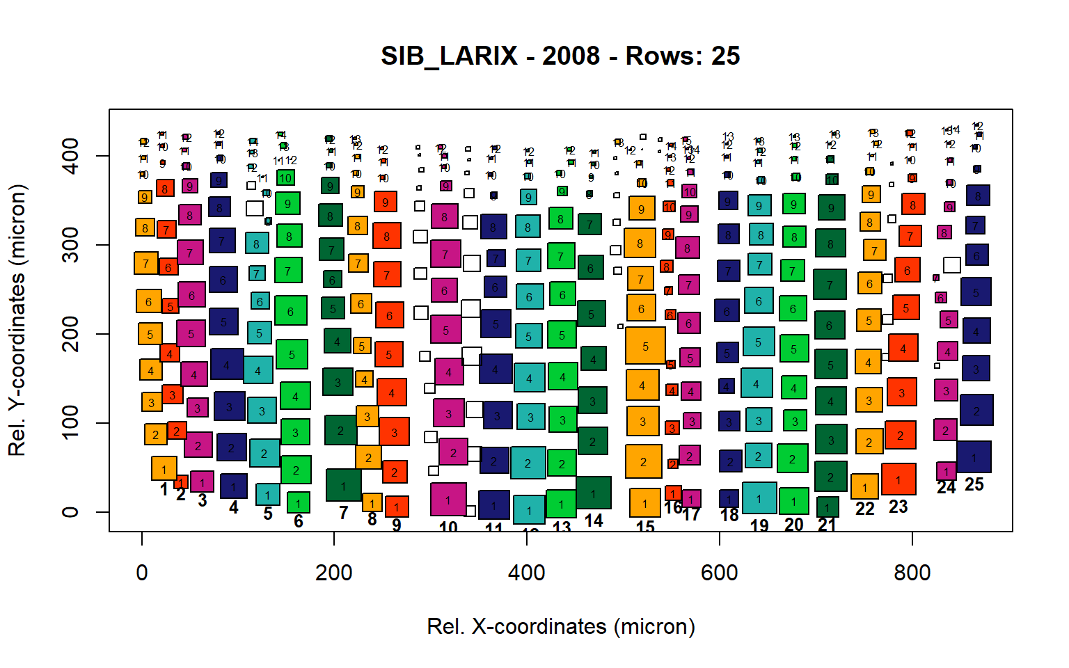
Figure 16: Standard plots generated by the write.output() function for Siberian Larix siberica (species="SIB_LARIX"), including 2007, 2008, 2009 and 2010.

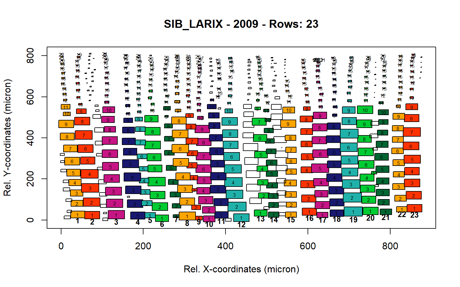
Figure 17: Standard plots generated by the write.output() function for Siberian Larix siberica (species="SIB_LARIX"), including 2007, 2008, 2009 and 2010.

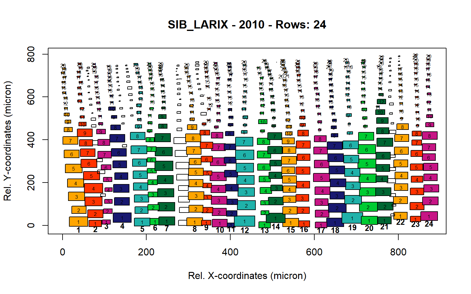
Figure 18: Standard plots generated by the write.output() function for Siberian Larix siberica (species="SIB_LARIX"), including 2007, 2008, 2009 and 2010.

Here we remove rows which are unsuitable.

# input

corrections<-data.frame(year=c(2010,2010,2010,2009,2009,2009,2009,2008,2008,2008,2008,2008,2008,
                               2007,2007,2007), row=c(19,15,9,6,11,14,17,5,6,14,17,24,15,2,8,14))
View(corrections)

# removing rows
for(i in c(1:nrow(corrections))){
    sib_larix[which(sib_larix[,"YEAR"]==corrections[i,1] &sib_larix[,"ROW"]==corrections[i,2] ),"POSITION"]<-rep(NA,length(sib_larix[which(sib_larix[,"YEAR"]==corrections[i,1]&sib_larix[,"ROW"]==corrections[i,2] ),"POSITION"]))
    sib_larix[which(sib_larix[,"YEAR"]==corrections[i,1] &sib_larix[,"ROW"]==corrections[i,2] ),"ROW"]<-rep(NA,length(sib_larix[which(sib_larix[,"YEAR"]==corrections[i,1]&sib_larix[,"ROW"]==corrections[i,2] ),"POSITION"]))}

# renumbering
SIB_LARIX<-write.output(sib_larix)

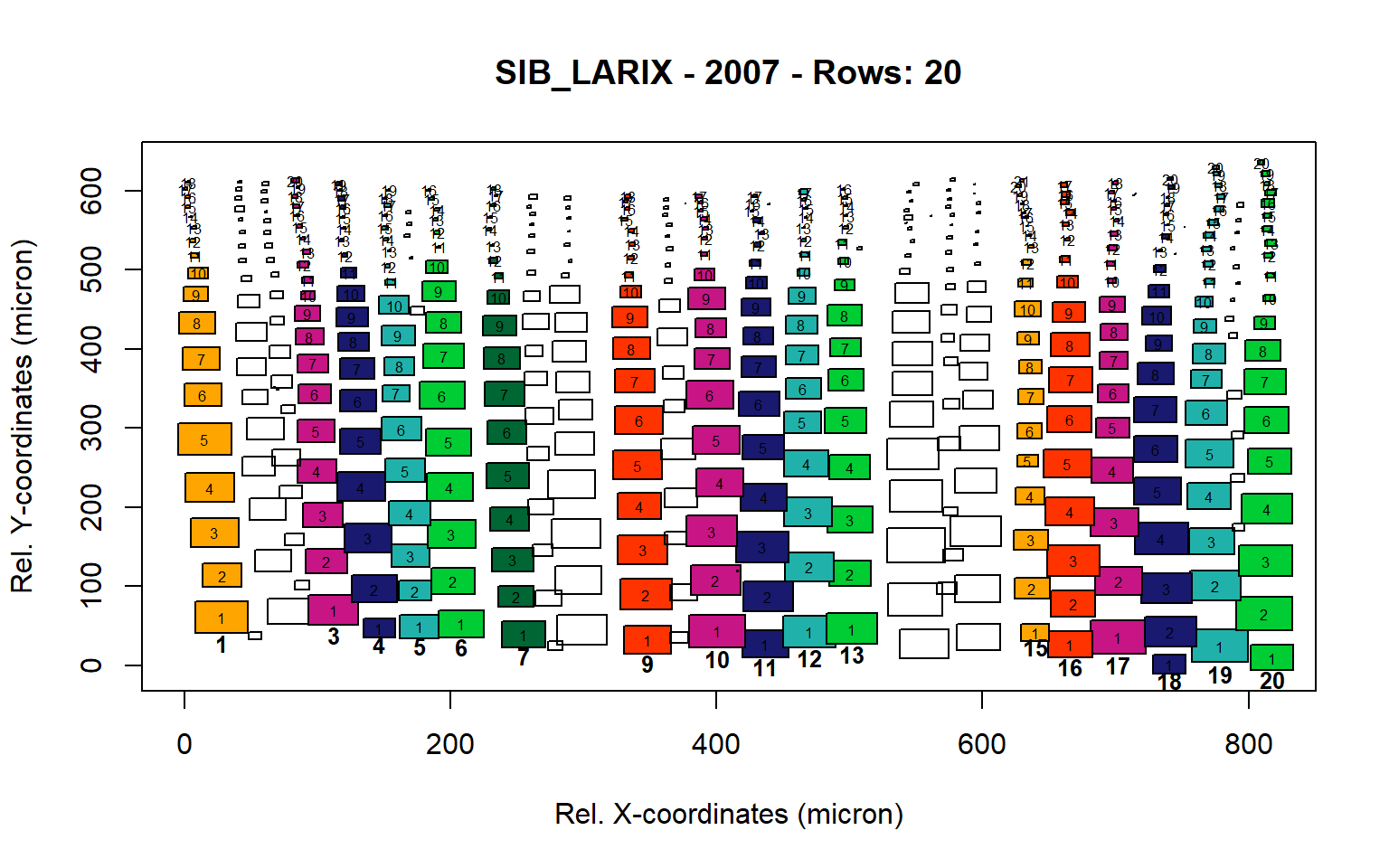
Figure 19: Standard plots generated by the write.output() function for Lotschental Picea abies (species="LOT_PICEA"), including 2007, 2008, 2009 and 2010.

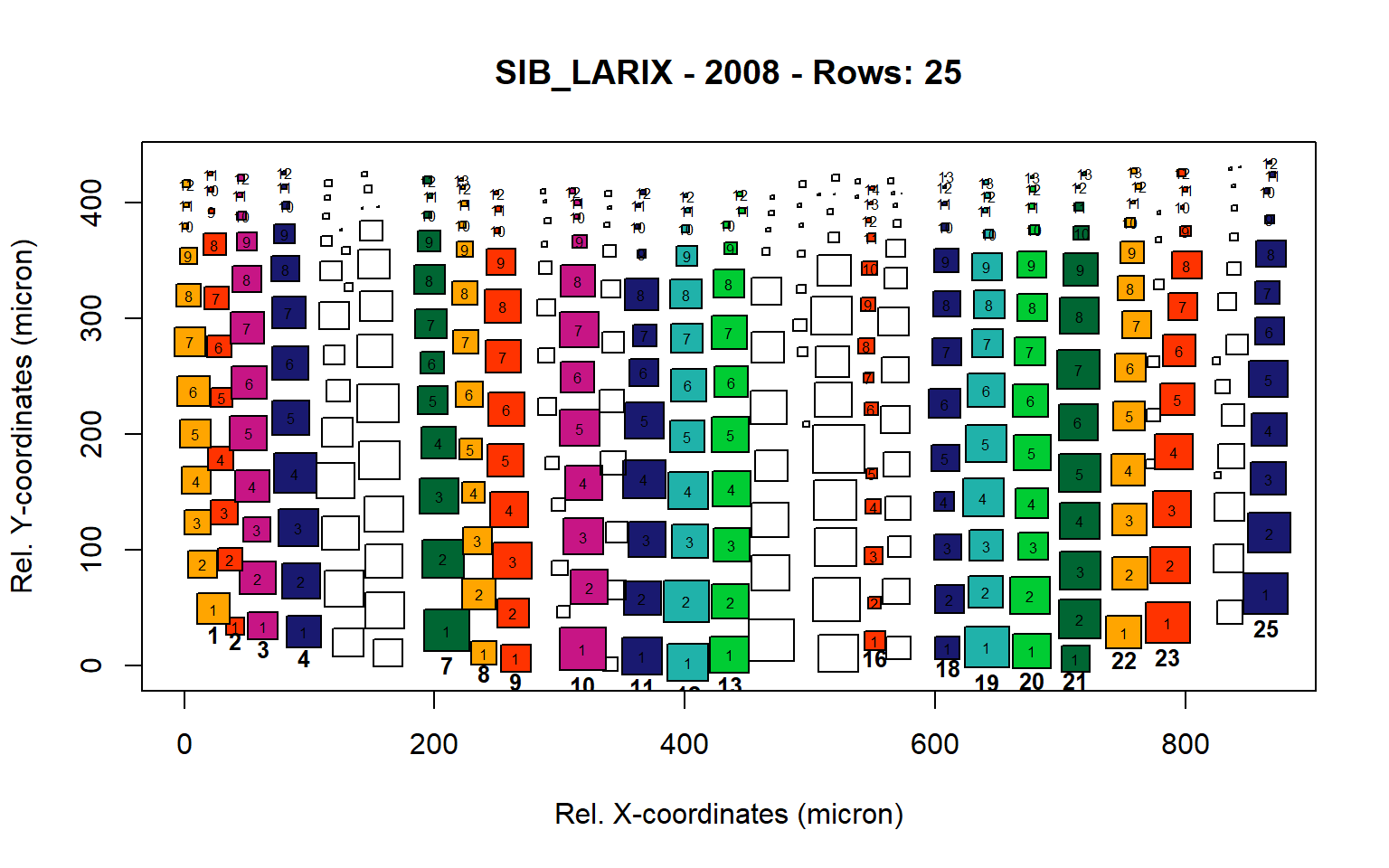
Figure 20: Standard plots generated by the write.output() function for Lotschental Picea abies (species="LOT_PICEA"), including 2007, 2008, 2009 and 2010.

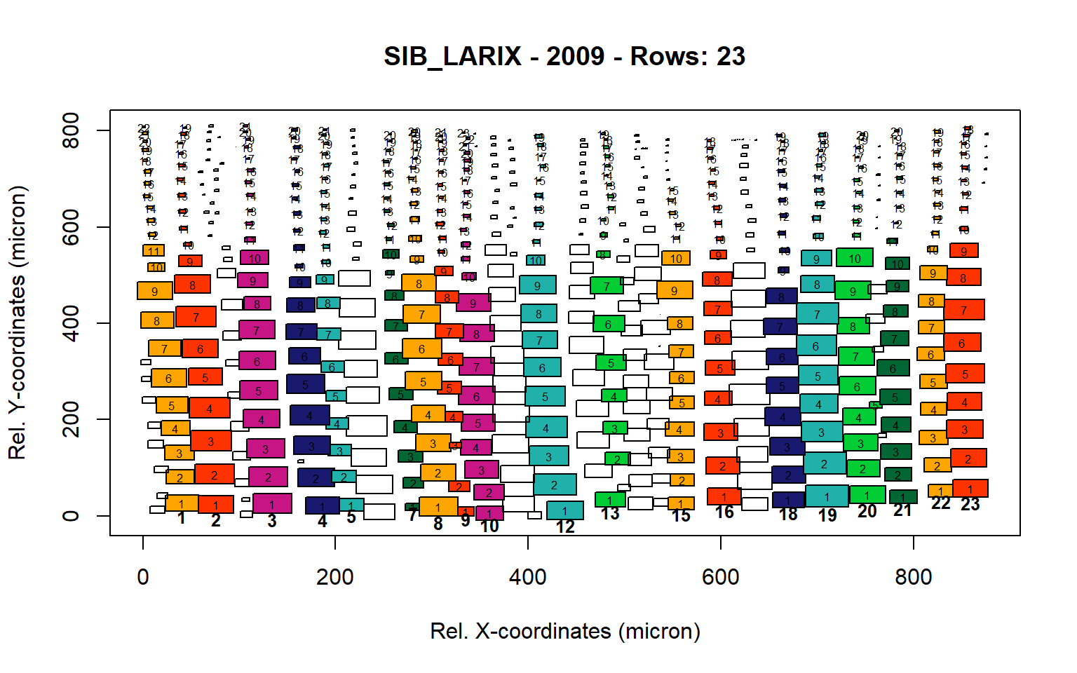
Figure 21: Standard plots generated by the write.output() function for Lotschental Picea abies (species="LOT_PICEA"), including 2007, 2008, 2009 and 2010.

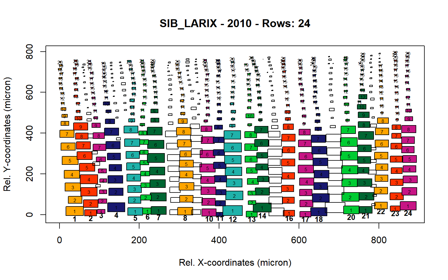
Figure 22: Standard plots generated by the write.output() function for Lotschental Picea abies (species="LOT_PICEA"), including 2007, 2008, 2009 and 2010.

for(i in c(1:length(unique(SIB_LARIX[,"YEAR"])))){
    row_id<-unique(SIB_LARIX[which(SIB_LARIX[,"YEAR"]==unique(SIB_LARIX[,"YEAR"])[i]) ,"ROW"],na.rm=TRUE)
    row_id<-na.omit(row_id[order(row_id)])
    for(j in c(1:length(row_id))){
        SIB_LARIX[which(SIB_LARIX[,"YEAR"]==unique(SIB_LARIX[,"YEAR"])[i] & SIB_LARIX[,"ROW"]==row_id[j]),"ROW"]<-j}}

# processing Lotschental Picea abies
input<-is.raptor(example.data(species="LOT_PICEA") , str = FALSE)
input<-input[which(input[,"YEAR"]>2006 &input[,"YEAR"]<2011),] #select years 2007-2010
aligned<-align(input,list=c(0.04,0.04,0,0))
first<-first.cell(aligned, frac.small = 0.5, yrs = FALSE, make.plot = FALSE)
output<-pos.det(first, swe = 0.5, sle = 3, ec = 1.75, swl = 0.25, sll = 5, lc = 10,prof.co = 1.5, max.cells = 0.5,
                yrs = FALSE, aligning = FALSE, make.plot = FALSE)
LOT_PICEA<-write.output(output)

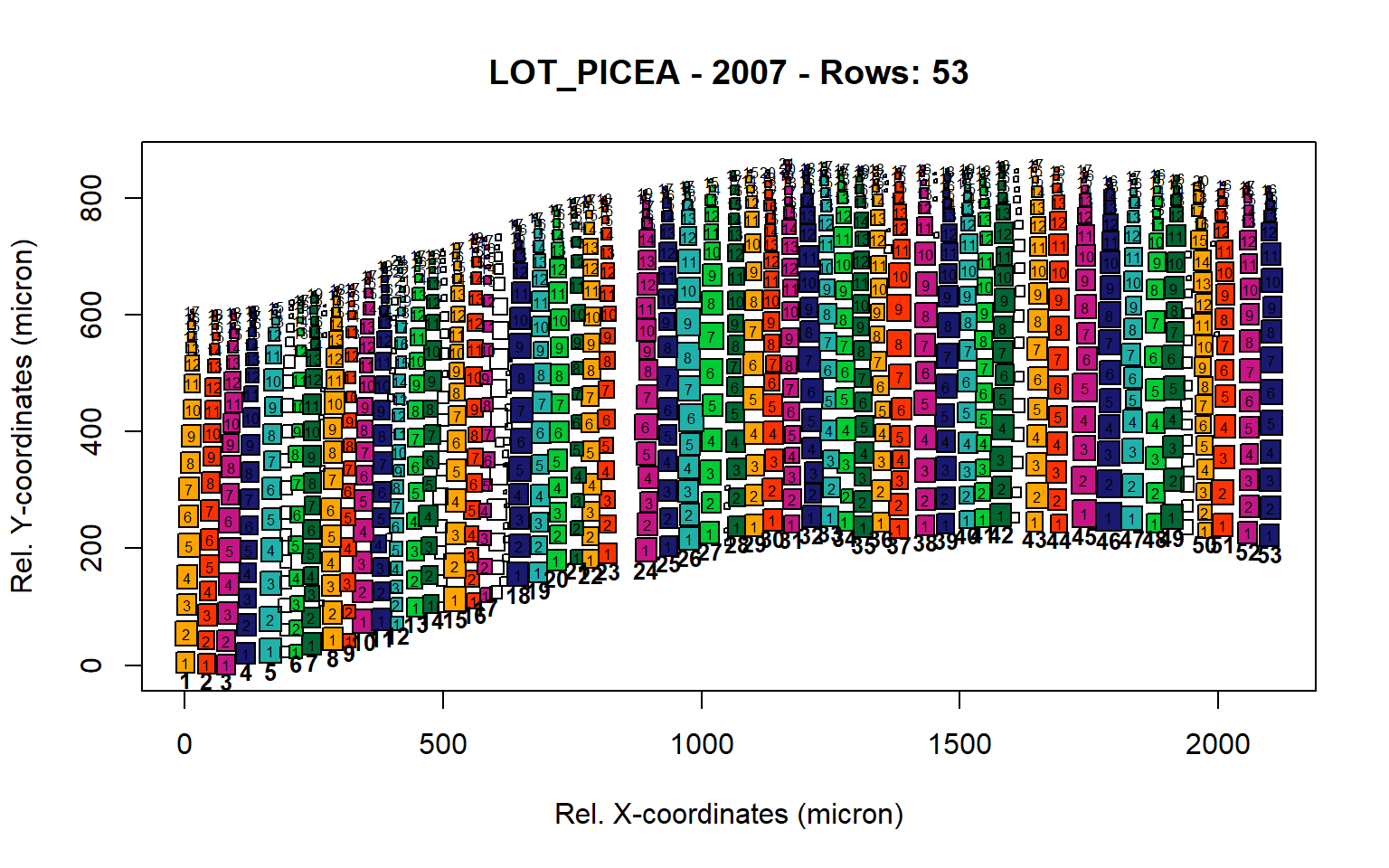
Figure 23: Standard plots generated by the write.output() function for Lotschental Picea abies (species="LOT_PICEA"), including 2007, 2008, 2009 and 2010.

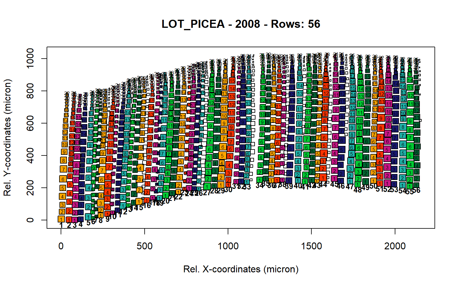
Figure 24: Standard plots generated by the write.output() function for Lotschental Picea abies (species="LOT_PICEA"), including 2007, 2008, 2009 and 2010.

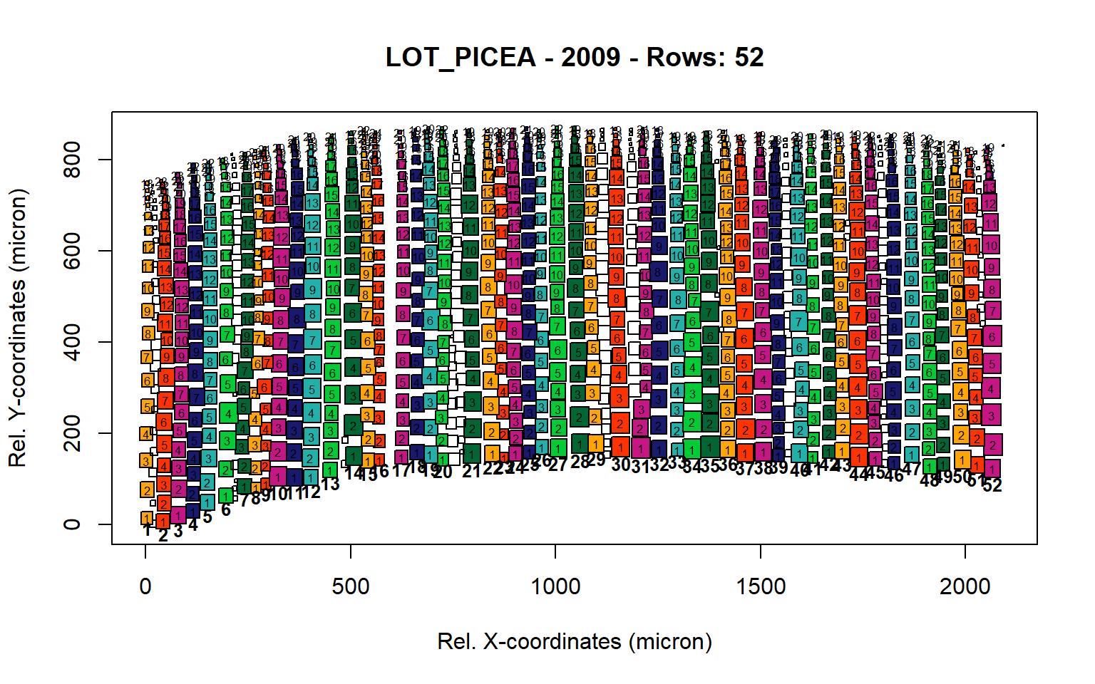
Figure 25: Standard plots generated by the write.output() function for Lotschental Picea abies (species="LOT_PICEA"), including 2007, 2008, 2009 and 2010.

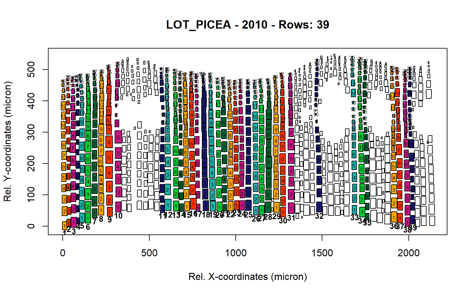
Figure 26: Standard plots generated by the write.output() function for Lotschental Picea abies (species="LOT_PICEA"), including 2007, 2008, 2009 and 2010.

Here we generate tracheidograms for all species.

#- loop for data preparation
sample<-c("LOT_PICEA","SIB_LARIX","MOUNT_PINUS","LOW_PINUS")
for(i in c(1:length(sample))){
    input<-get(sample[i])
    years<-unique(as.numeric(input$YEAR))
    for(j in c(1:length(years))){
        select<-input[which(input["YEAR"]==years[j]),]

        #- preparing data
        lumen<-na.omit(data.frame(gram=select[,"ROW"],lumen.wall="l",order=select[,"POSITION"], area=select[,"CA"]))
        wall<-na.omit(data.frame(gram=select[,"ROW"],lumen.wall="w",order=select[,"POSITION"], area=select[,"CWTALL"]))
        gram<-rbind(lumen,wall)
        gram<-gram[order(gram[,"gram"]),]
        gram[,"gram"]<-as.integer(gram[,"gram"])

        #- determining mean maximum cells
        max.cells<-NA
        for(z in c(1:max(gram[,"gram"]))){gram[which(gram[,"gram"]==unique(gram[,"gram"])[z]),]
            max.cells[z]<-max(gram[which(gram[,"gram"]==unique(gram[,"gram"])[z]),"order"])}
        mean.cells<-round(mean(max.cells))

        #- apply standardization
        output<-with(gram,standz.all(traq=area, series=gram,wl=lumen.wall, w.char="w", G=mean.cells))
        lumen.mean<-colMeans(output$data.stdz[output$which.l,])
        wall.mean<-colMeans(output$data.stdz[output$which.w,])

        #- generate output and store data
        output<-data.frame(ID=sample[i],YEAR=years[j],POSITION=c(1:mean.cells) ,LUMEN= lumen.mean,
                           WALL= wall.mean)
        if(i==1&j==1){final<-output}else{final<-rbind(final,output)}}}

#Here we perform an inter-species comparison on multi-annual tracheidograms, by plotting median radial file differences between years and species.

#- plotting of output
layout(matrix(c(1,3,5,7,2,4,6,8),nc=4, byrow = TRUE))
par(oma=c(5,5,1,1))
par(mar=c(0,1,1,0))
lumen.lim<-2000
wall.lim<-11
colour<-c("darkgreen","darkorange","palegreen","greenyellow")
thickness<-c(1,1,2,2)
type<-c(2,1,2,1)
for(i in c(1:length(sample))){
    select<-final[which(final[,"ID"]==sample[i]),]
    plot(1,1,type="l",ylab="",col="white",xlab="",yaxt="n",xaxt="n",ylim=c(0,lumen.lim),xlim=c(1,max(select[,
                                                                                                            "POSITION"])))
    axis(side=1,labels=FALSE)
    axis(side=2,las=2,labels=FALSE)
    if(i==4){abline(v=seq(0,100,10),col="grey",lty=3)}else{abline(v=seq(0,100,5),col="grey",lty=3)}
    box()
    if(i==1){mtext(side=2, expression("Lumen area ("*micron^2*")"),padj=-2)
        axis(side=2,las=2)
        legend("topleft",c("2007","2008","2009","2010"),
               lty=c(2,1,2,1),lwd=c(1,1,2,2),col=c("black","black","black","black"),bty="n")}
    for(j in c(1:length(unique(select[,"YEAR"])))){
        lines(select[which(select[,"YEAR"]==unique(select[,"YEAR"])[j]),"POSITION"],select[which(select[,"YEAR"]==unique(select[,"YEAR"])[j]),"LUMEN"],col=colour[i],lwd=thickness[j],lty=type[j])}
    plot(1,1,type="l",ylab="",col="white",xlab="",yaxt="n",xaxt="n",ylim=c(1.5,wall.lim),xlim=c(1,max(select[,
                                                                                                             "POSITION"])))
    axis(side=1)
    axis(side=2,las=2,labels=FALSE)
    if(i==4){abline(v=seq(0,100,10),col="grey",lty=3)}else{abline(v=seq(0,100,5),col="grey",lty=3)}
    box()
    if(i==1){mtext(side=2, expression("Cell wall thickness ("*micron^2*")"), padj=-2)
        axis(side=2,las=2)
        legend("topleft",c("Picea abies","Larix sibirica","Pinus cembra","Pinus sylvestris"),
               lty=c(1,1,1,1),lwd=c(2,2,2,2),col=colour,bty="n",text.font=c(3,3,3,3))}
    for(j in c(1:length(unique(select[,"YEAR"])))){
        lines(select[which(select[,"YEAR"]==unique(select[,"YEAR"])[j]),"POSITION"],select[which(select[,"YEAR"]==unique(select[,"YEAR"])[j]),"WALL"],col=colour[i],lwd=thickness[j],lty=type[j])}}
mtext(side=1,"Cell position (#)",padj=3,outer=TRUE)

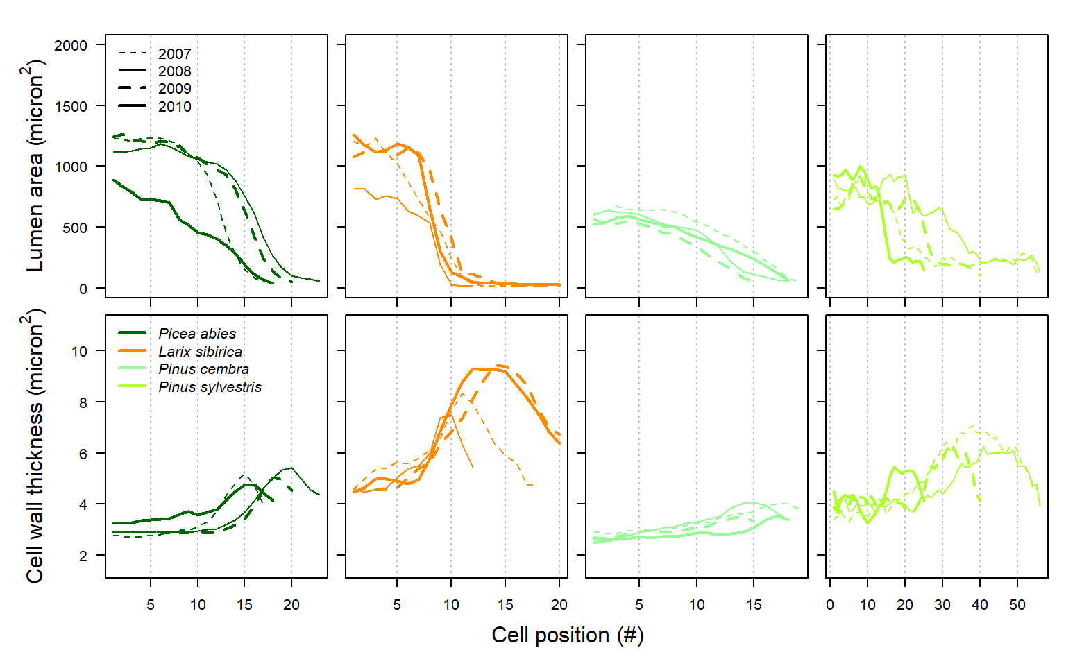
Figure 27: Comparison of individual tracheidograms within a single annual ring (upper graph) and mean tracheidogram among years and species (lower graph) as obtained with RAPTOR using the example data (including Picea abies, Larix siberica, Pinus cembra and Pinus sylvestris; see example.data ()).

The increased robustness will benefit a multitude of studies that require representative cell-based anatomical tree-ring profiles for gymnosperm species, as is often the case when modeling tree-ring formation, structure and functioning.