Sectoral analyses of radial growth profiles (SECTOR)
A workflow for diffuse-porous species
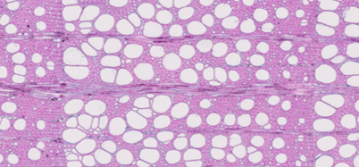 Image credit: R. Peters
SECTOR Workflow
1. Background
Although methods are highly advanced for determining radial progression of wood anatomical properties for coniferous species (see RAPTOR), no methods are yet available for more complex wood structures (i.e., angiosperm species). More specifically, defining the cell order (as done in tracheidograms) is difficult for angiosperm species (i.e., Fagus sylvatica) and thus requires an alternative approach for studying intra-annual wood anatomical properties and their dynamics. Here we introduce SECTOR, an R script capable of applying a sectoral approach, where wood anatomical measurements obtained from ROXAS are automatically assigned to a specified sector (or bin), accounting for the ring shape and rotation. SECTOR also allows for automatically providing intra-annual data on key wood anatomical parameters, while correcting for gaps in the area of interest (i.e., caused by cracks due to cutting). Quantitative wood anatomical analysis can be used in SECTOR to determine cell-specific properties of wood cores to quantify the bin specific wood anatomical parameters, including high-resolution measurements of hydraulic parameters (i.e., derived from cell number and lumen size). Additionally, this approach allows us to ascertain which wood anatomical properties contribute most to the intra-annual variability in wood density (e.g., lumen area to xylem conductivity). SECTOR is envisioned to be incorporated into the RAPTOR package as an individual function. Although this function is still under development, we provide the raw code with an example below. The code is structured in such a way that it is easy to test within R, despite the lack of properly constructed functions with error messages. As such, please utilize this code with care and follow the data input requirements presented with the example data.
2. Set-up steps
#install package if necessary
packages <- (c("zoo"))
install.packages(setdiff(packages, rownames(installed.packages())))
library(zoo)
##
## Attaching package: 'zoo'
## The following objects are masked from 'package:base':
##
##     as.Date, as.Date.numeric
3. Import data
The data presented here originates from a well-monitored forests near Basel, Switzerland ($ 47^\circ 28'7''N$, $ 7^\circ 30'8''E $, $ 550~m $ above sea level). The average annual air temperature is $ 10.5^\circ C$ with an annual total precipitation of $ 990~mm $, where the growing season ranges from end of April to early October. The forest stand is dominated by Fagus sylvatica L. and Quercus petraea (Matuschka) Liebl., with an age range of 80-130 years. At the stand level, tree height ranges from $ 30-35~m $, tree (diameter at breast height $ > 10~cm $) density is 415 trees $ ha^{-1} $, and the basal area approximates $ 46~m^2 ha^{-1} $. Other species present within the stand include Abies alba Mill., Larix decidua Mill., Picea abies (L.) Karst, Pinus sylvestris L., and Carpinus betulus L. On January 2019, wood cores of ca. $ 12~cm $ length were taken from a Fagus sylvatica tree (using a increment borer; Haglöf, Sweden). For the wood core, $ 10-12~micron $ thick micro-sections were cut using a rotatory microtome (Leica RM2245, Leica Biosystems, Nussloch, Germany). The thin sections was stained with safranin and astrablue, and fixed on glass slides using Canada balsam Digital images of radial anatomical properties (fibres and vessels) were taken from the thin sections for each sapwood ring using a slide-scanner (Axio Scan Z1, Zeiss, Germany). ROXAS combined with Image-Pro Plus (Media Cybernetics, Rockville, MD, USA), allowed us to detect fibres and vessels.
Below one can see the ROXAS output structure required for the analysis.
#cell specific ROXAS output
sel_raw<-cell<-read.table(
  "https://raw.githubusercontent.com/deep-org/materials/main/data/measurements/02_sector/HOF_FASY_Output_Cells.txt",
  header=T,sep="\t")
head(sel_raw)
##              ID CID YEAR    LA RADDIST   ANGLE    XCAL     YCAL XPIX YPIX
## 1 HOF_FASY_2A_2   1 2009 12.44 66159.6 179.373  723.80 66155.64 4141    8
## 2 HOF_FASY_2A_2   2 2009 13.89 66162.0 180.772 -891.15 66155.95  479    9
## 3 HOF_FASY_2A_2   3 2009 10.18 66157.9 180.363 -419.45 66156.59 1549   10
## 4 HOF_FASY_2A_2   4 2009 10.10 66156.0 180.241 -277.83 66155.46 1870    8
## 5 HOF_FASY_2A_2   5 2009 17.55 66157.0 179.678  371.83 66155.92 3343    9
## 6 HOF_FASY_2A_2   6 2009  7.50 66162.7 179.153  977.75 66155.48 4717    8
##   RADDISTR RRADDISTR NBRNO NBRID NBRDST  ASP MAJAX          KH AOI CWTPI CWTBA
## 1        8      1.70     0  <NA>   <NA> 1.99 68.23 4.31272e-15  NA    NA    NA
## 2       10      4.12     0  <NA>   <NA> 1.52 61.65 6.54479e-15  NA    NA    NA
## 3        6      2.00     0  <NA>   <NA> 2.20 29.61 2.65663e-15  NA    NA    NA
## 4        4      1.17     0  <NA>   <NA> 1.48 75.70 3.51283e-15  NA    NA    NA
## 5        5      1.20     1    43   7.31 1.15 85.76 1.19448e-14  NA    NA    NA
## 6       11      2.25     0  <NA>   <NA> 1.79 43.62 1.70380e-15  NA    NA    NA
##   CWTLE CWTRI CWTTAN CWTRAD CWTALL RTSR CTSR   DH DRAD DTAN TB2 CWA RWD
## 1    NA    NA     NA     NA     NA   NA   NA 3.57 2.89 5.47  NA  NA  NA
## 2    NA    NA     NA     NA     NA   NA   NA 4.03 3.55 4.99  NA  NA  NA
## 3    NA    NA     NA     NA     NA   NA   NA 3.13 4.26 3.04  NA  NA  NA
## 4    NA    NA     NA     NA     NA   NA   NA 3.45 2.96 4.35  NA  NA  NA
## 5    NA    NA     NA     NA     NA   NA   NA 4.70 4.42 5.05  NA  NA  NA
## 6    NA    NA     NA     NA     NA   NA   NA 2.85 2.72 3.51  NA  NA  NA
#ring specific ROXAS output
sel_rw<-ring<-read.table(
  "https://raw.githubusercontent.com/deep-org/materials/main/data/measurements/02_sector/HOF_FASY_Output_Rings.txt",
  header=T,sep="\t")
head(sel_rw)
##              ID YEAR    RA  MRW MINRW MAXRW MRADDIST  CNO      CD   CTA  RCTA
## 1 HOF_FASY_2A_2 2009 0.816  373   229   494      373 1614 1976.88 0.127 15.61
## 2 HOF_FASY_2A_2 2010 3.133 1411  1390  1459     1794 3598 1148.59 1.248 39.83
## 3 HOF_FASY_2A_2 2011 2.086  941   920   964     2740 2759 1322.67 0.781 37.44
## 4 HOF_FASY_2A_2 2012 5.307 2400  2329  2471     5145 7019 1322.51 1.827 34.41
## 5 HOF_FASY_2A_2 2013 4.378 1984  1912  2027     7126 5721 1306.64 1.520 34.72
## 6 HOF_FASY_2A_2 2014 1.695  768   739   807     7897 2758 1626.93 0.599 35.35
##   MLA MINLA MAXLA          KH       KS RVGI RVSF RGSGV AOIAR RAOIAR CWTPI CWTBA
## 1  79     5  3496 6.73635e-09 0.008251   NA   NA    NA    NA     NA    NA    NA
## 2 347     5  8564 1.78135e-07 0.056866   NA   NA    NA    NA     NA    NA    NA
## 3 283     5  5699 7.81140e-08 0.037448   NA   NA    NA    NA     NA    NA    NA
## 4 260     5  7826 2.24346e-07 0.042271   NA   NA    NA    NA     NA    NA    NA
## 5 266     5  7113 2.00392e-07 0.045768   NA   NA    NA    NA     NA    NA    NA
## 6 217     5  6482 6.40089e-08 0.037759   NA   NA    NA    NA     NA    NA    NA
##   CWTLE CWTRI CWTTAN CWTRAD CWTALL RTSR CTSR    DH   DH2  DRAD DTAN TB2 CWA RWD
## 1    NA    NA     NA     NA     NA   NA   NA 47.56 20.32  5.73 5.71  NA  NA  NA
## 2    NA    NA     NA     NA     NA   NA   NA 74.34 37.65 10.87 9.54  NA  NA  NA
## 3    NA    NA     NA     NA     NA   NA   NA 62.92 32.75 10.08 9.88  NA  NA  NA
## 4    NA    NA     NA     NA     NA   NA   NA 69.24 33.74  9.52 8.27  NA  NA  NA
## 5    NA    NA     NA     NA     NA   NA   NA 72.03 34.51  9.50 8.23  NA  NA  NA
## 6    NA    NA     NA     NA     NA   NA   NA 65.89 31.17  8.70 8.28  NA  NA  NA
4. Define parameters
To feed the loop which will perform the sector analysis, one has to provide relevant parameters which aid in fine-tuning the processing. Often these parameters are subjectively defined by the user.
#Relevant parameters:
#A character indicating the sample and site name
name<-"HOF_FASY"
sample<-"HOF"
site<-"HOF"
tree<-"FASY_1"
#Species
species<-"Fagus sylvatica"

#A numeric value indicating that the bin cannot be x times smaller in length than the selected bin size
bin_min<-10
#A numeric value indicating minimum size for a vessel (i.e., beech = 200 square micron; oak = 400 square micron)
vessel_size<-200
#A numeric value indicating the minimum cell size included within the analysis in square micron
smallest_cell<-15
#A numeric value indicating the maximum cell size included within the analysis in square micron
biggest_cell<-15000

#A 0 or 1 nominator indicating if the sample needs to be aligned (according to the align() function in RAPTOR) to the ring boundary (TRUE= 1)
rotate<-1
#A logical flag indicating whether we utilize a circle (non-coniferous="diff" or "ring") or square (coniferous="con")
wood_type <- "diff"

#A numeric value identifying an the minimum width of an empty space of x micron which will be considered as a ray
ray_min <- 100
#A numeric value identifying an the maximum width of an empty space of x micron which will be considered as a ray
ray_max <- 300  #'  an empty space of 50 micron will be considered as a ray

#A numeric value which provides an estimation of the average cell wall thickness
cwt<-4
This parameter is needed as cell wall thickness is often not correctly detected for diffuse-porous species (due to missing fiber cells).
#A numeric value indicating the start and end year of the data
end_year<-2018
start_year<-2018
Within this example we only show one year. Yet this can easily be adjusted.
5. Sector analysis
After defining all parameters, one can start processing of the data utilizing a sector approach. First, only cells are considered which the indicated size.
#remove large or small cells
sel_raw<-sel_raw[which(sel_raw[,"LA"]>=smallest_cell&sel_raw[,"LA"]<=biggest_cell),]
Below a for loop is provided which can run the analyses for multiple years per sample. Within this loop several actions are performed, including:
- aligning the sample,
- correction for the shape of the ring boundary and
- isolating the bins (or sectors).
Within each bin both ray areas and empty spaces are detected. Non-ray assigned empty spaces (within the detected area of interest) are filled with the missing number of cells defined with the medium properties of the fibers (or tracheids in case of conifers). One thus has to make sure that most vessels for both diffuse- and ring-porous species have been detected.
#initiating the loop
for(y in c(1:length(c(start_year:end_year)))){
label<-paste0(site," | ",species," | ",tree," | ",c(start_year:end_year)[y])
print(label)
if(length(which(unique(sel_raw$YEAR)==c(start_year:end_year)[y]))==0){
print(paste("error:",label))
next}
sel<-sel_raw[which(sel_raw$YEAR==c(start_year:end_year)[y]),]
#mean length of a bin defined by the largest cell within the sample
bin_size<-ceiling(quantile((sel$DRAD),probs=c(0.95))) #' width of each bin
if(wood_type=="rin"){
bin_size<-ceiling(quantile((sel$DRAD),probs=c(1))) #' width of each bin
}
if(wood_type=="dif"){
bin_size<-ceiling(quantile((sel$DRAD),probs=c(0.99))) #' width of each bin
}
print(paste0("bin_size: ",bin_size))
sel$XCAL<-sel$XCAL-min(sel$XCAL)+1000
sel$YCAL<-sel$YCAL-min(sel$YCAL)+1000
#project the ring boundary cells
ring_position<-data.frame(xcal=seq(min(sel$XCAL)-0.5,max(sel$XCAL)+0.5,by=5),ycal=NA,dist=NA,ypos=NA)
for(r in c(1:nrow(ring_position))){
options<-sel[which(sel$XCAL>=ring_position[r,1]&sel$XCAL<ring_position[r+1,1]),]
if(nrow(options)==0){
ring_position[r,c(2:4)]<-NA
}else{
ring_position[r,2]<-options[which(options$YCAL==min(options$YCAL)),"YCAL"]
ring_position[r,3]<-options[which(options$YCAL==min(options$YCAL)),"RADDISTR"]
ring_position[r,4]<-ring_position[r,2]-ring_position[r,3]}
}
ring<-na.omit(ring_position)[,c(1,4)]
model<-lm(ring$ypos~ring$xcal)
#rotate sample
y_model<-as.numeric(c(model$coefficients[2]*0+model$coefficients[1],model$coefficients[2]*100+model$coefficients[1]))
change_angle<-atan((y_model[2]-y_model[1])/(100-0))*(180/pi)
#upper ring detection
ring_position_last<-data.frame(xcal=seq(min(sel$XCAL)-0.5,max(sel$XCAL)+0.5,by=5),ycal=NA,dist=NA,ypos=NA)
for(r in c(1:nrow(ring_position_last))){
options<-sel[which(sel$XCAL>=ring_position_last[r,1]&sel$XCAL<ring_position_last[r+1,1]),]
if(nrow(options)==0){
ring_position_last[r,c(2:4)]<-NA
}else{
ring_position_last[r,2]<-options[which(options$YCAL==max(options$YCAL)),"YCAL"]
ring_position_last[r,3]<-(options[which(options$YCAL==max(options$YCAL)),"RADDISTR"]/options[which(options$YCAL==max(options$YCAL)),"RRADDISTR"])*
(100-options[which(options$YCAL==max(options$YCAL)),"RRADDISTR"])
ring_position_last[r,4]<-ring_position_last[r,2]+ring_position_last[r,3]}}
ring_last<-na.omit(ring_position_last)[,c(1,4)]
raw<-cbind(sel[,c("XCAL","YCAL")],c=1)
colnames(ring)<-c("XCAL","YCAL")
colnames(ring_last)<-c("XCAL","YCAL")
raw<-rbind(raw,cbind(ring,c=2))
raw<-rbind(raw,cbind(ring_last,c=3))
output<-raw
if(rotate==1){
r<-sqrt(raw[,"XCAL"]^2+raw[,"YCAL"]^2)
current_angle<-atan(raw[,"XCAL"]/raw[,"YCAL"])*(180/pi)
new_angle<-current_angle+change_angle
x_new<-r*sin(new_angle*(pi/180))
y_new<-r*cos(new_angle*(pi/180))
output[,"XCAL"]<-x_new
output[,"YCAL"]<-y_new
output[,"XCAL"]<-output[,"XCAL"]-min(output[,"XCAL"])
output[,"YCAL"]<-output[,"YCAL"]-min(output[,"YCAL"])
sel$XCAL<-output[which(output[,3]==1),"XCAL"]
sel$YCAL<-output[which(output[,3]==1),"YCAL"]
}
#calculate distance to ring boundary
layout(matrix(c(1,1,1,
1,1,1,
2,2,3,
2,2,3),nc=3, byrow = TRUE))
par(oma=c(4,4,4,4))
par(mar=c(5,2,2,2))
plot(sel$XCAL,sel$YCAL,xlim=c(min(sel$XCAL),max(sel$XCAL)+((max(sel$XCAL)-min(sel$XCAL))*0.1)),pch=16,cex=1,yaxt="n",ylab="",xlab="",xaxt="n")
mtext(side=3,outer=F,label,padj=-0.5,font=2,col="darkgrey",cex=1.2)
legend("bottomright",c("Cells","Rings"),
pch=c(16,NA),lty=c(NA,1),lwd=c(NA,2),pt.cex=c(1,NA),col=c("black","darkgrey"),
bty="n",cex=1.2)
legend("topright","(a)",bty="n",cex=2)
ring_cor<-output[which(output[,3]==2),c(1,2)]
ring_last_cor<-output[which(output[,3]==3),c(1,2)]
lines(ring_cor$XCAL,ring_cor$YCAL,col="darkgrey",lwd=2)
lines(ring_last_cor$XCAL,ring_last_cor$YCAL,col="darkgrey",lwd=2)
#finishing rings
ring_cor$XCAL<-round(ring_cor$XCAL)
ring_cor$YCAL<-floor(ring_cor$YCAL)
ring_final<-data.frame(XCAL=seq(-10000,max(ring_cor[,1])+10000,1),YCAL=NA)
for(o in c(1:nrow(ring_final))){
add<-(ring_cor[which(ring_cor$XCAL==ring_final[o,1]),"YCAL"])
if(length(add)==0){ring_final[o,2]<-NA}else{ring_final[o,2] <-min(add)}}
ring_final[,2]<-na.approx(ring_final[,2],na.rm=FALSE)
add_min<-cbind(c(round(min(sel$XCAL)-10000):min(na.omit(ring_final)[,1])-1),na.omit(ring_final)[1,2])
add_max<-cbind(c(max(na.omit(ring_final)[,1])+1):(round(max(sel$XCAL))+10000),na.omit(ring_final)[nrow(na.omit(ring_final)),2])
colnames(add_min)<-c("XCAL","YCAL")->colnames(add_max)
ring_final<-rbind(add_min,na.omit(ring_final),add_max)
ring_last_cor$Xcal<-round(ring_last_cor$XCAL)
ring_last_cor$Ycal<-floor(ring_last_cor$YCAL)
ring_last_final<-data.frame(XCAL=seq(-10000,max(ring_cor[,1])+10000,1),YCAL=NA)
for(o in c(1:nrow(ring_last_final))){
add<-(ring_last_cor[which(ring_last_cor$Xcal==ring_last_final[o,1]),"YCAL"])
if(length(add)==0){ring_last_final[o,2]<-NA}else{ring_last_final[o,2] <-min(add)}}
ring_last_final[,2]<-na.approx(ring_last_final[,2],na.rm=FALSE)
add_min<-cbind(c(round(min(sel$XCAL)-10000):min(na.omit(ring_last_final)[,1])-1),na.omit(ring_last_final)[1,2])
add_max<-cbind(c(max(na.omit(ring_last_final)[,1])+1):(round(max(sel$XCAL))+10000),na.omit(ring_last_final)[nrow(na.omit(ring_last_final)),2])
colnames(add_min)<-c("XCAL","YCAL")->colnames(add_max)
ring_last_final<-rbind(add_min,na.omit(ring_last_final),add_max)
#average ring width
mu_rw<-mean(ring_last_final[,2]-ring_final[,2],na.rm=TRUE)
#standardize towards the ring percentage
low<-ring_final[match(round(sel$XCAL),ring_final$XCAL),"YCAL"]
high<-ring_last_final[match(round(sel$XCAL),ring_last_final$XCAL),"YCAL"]
DISTANCE<-(sel$YCAL-low)/(high-low)*mu_rw
#calculate radial distance
sel<-cbind(sel,DISTANCE)
par(mar=c(2,2,0,0))
plot(sel$XCAL,sel$DISTANCE,col="grey",pch=16,cex=0.3,xlim=c(min(sel$XCAL),(max(sel$XCAL)+((max(sel$XCAL)-min(sel$XCAL))*0.3))),ylim=c(0,(max(sel$DISTANCE)+((max(sel$DISTANCE)-min(sel$DISTANCE))*0.15) )),yaxt="n")
axis(side=2,las=2)
axis(side=3)
mtext(side=1,expression(italic(X)[cal]*" ["*mu*"m]"),padj=3)
mtext(side=2,expression(italic(Y)[cal]*" ["*mu*"m]"),padj=-3)
mtext(side=3,expression(italic(X)[cal]*" ["*mu*"m]"),padj=-2)
#determine bin sizes
new_rw<-max(DISTANCE)
print(paste("Micron difference in rw = ",round(new_rw-mu_rw,3),sep=""))
n_bin<-floor(new_rw/bin_size)
bins<-c(seq(0,bin_size*n_bin,bin_size),(new_rw+0.00001))
box()
#add vessel types
sel$Cell.type<-1
sel[which(sel$LA<vessel_size),"Cell.type"]<-0
#bin analyses (edge effect removal)
bound<-data.frame(y=bins[],x_min=NA,x_max=NA)
for(b in c(1:(length(bins)-1))){
#' vessels
bin_sel<-sel[which(sel$DISTANCE>=bins[b]&sel$DISTANCE<bins[b+1]),]
ves_sel<-bin_sel[which(bin_sel$Cell.type==1),]
if(nrow(ves_sel)>0){
quant<-0.02
if(wood_type=="dif"){quant<-0.02}
bound[b,2]<-quantile(ves_sel$XCAL,probs=c(quant,1-quant))[c(1)]
bound[b,3]<-quantile(ves_sel$XCAL,probs=c(quant,1-quant))[c(2)]
}else{
bound[b,2]<-quantile(bin_sel$XCAL,probs=c(quant,1-quant))[c(1)]
bound[b,3]<-quantile(bin_sel$XCAL,probs=c(quant,1-quant))[c(2)]
}
}
if(wood_type!="rin"&nrow(bound)!=2){
if(length(c(rollmean(na.fill(bound[,2], "extend"),k=5)[1],rollmean(na.fill(bound[,2], "extend"),k=5)[1],rollmean(na.fill(bound[,2], "extend"),k=5),rollmean(na.fill(bound[,2], "extend"),k=5)[length(rollmean(na.fill(bound[,2], "extend"),k=5))],rollmean(na.fill(bound[,2], "extend"),k=5)[length(rollmean(na.fill(bound[,2], "extend"),k=5))]))==0){
bound$roll_x_min<-min(sel$XCAL,na.rm=T)
bound$roll_x_max<-max(sel$XCAL,na.rm=T)
}else{
bound$roll_x_min<-c(rollmean(na.fill(bound[,2], "extend"),k=5)[1],rollmean(na.fill(bound[,2], "extend"),k=5)[1],rollmean(na.fill(bound[,2], "extend"),k=5),rollmean(na.fill(bound[,2], "extend"),k=5)[length(rollmean(na.fill(bound[,2], "extend"),k=5))],rollmean(na.fill(bound[,2], "extend"),k=5)[length(rollmean(na.fill(bound[,2], "extend"),k=5))])
bound$roll_x_max<-c(rollmean(na.fill(bound[,3], "extend"),k=5)[1],rollmean(na.fill(bound[,3], "extend"),k=5)[1],rollmean(na.fill(bound[,3], "extend"),k=5),rollmean(na.fill(bound[,3], "extend"),k=5)[length(rollmean(na.fill(bound[,3], "extend"),k=5))],rollmean(na.fill(bound[,3], "extend"),k=5)[length(rollmean(na.fill(bound[,3], "extend"),k=5))])
bound[which(is.na(bound$x_min)==TRUE),"x_min"]<-na.omit(bound[,"x_min"])[length(na.omit(bound[,"x_min"]))]
bound[which(is.na(bound$x_max)==TRUE),"x_max"]<-na.omit(bound[,"x_max"])[length(na.omit(bound[,"x_max"]))]
bound$roll_x_min<-apply(bound[,c(2,4)], 1, max)
bound$roll_x_max<-apply(bound[,c(3,5)], 1, min)
}
}else{
bound$roll_x_min<-min(sel$XCAL,na.rm=T)
bound$roll_x_max<-max(sel$XCAL,na.rm=T)
}
for(b in c(1:(length(bins)-1))){
polygon(c(bound[b,"roll_x_min"],bound[b,"roll_x_max"],bound[b,"roll_x_max"],bound[b,"roll_x_min"]),c(bound[b,"y"],bound[b,"y"],bound[b+1,"y"],bound[b+1,"y"]),
col=rgb(0,0,0,0))
}
#bin analysis
for(b in c(1:(length(bins)-1))){
#theoretical cell wall thickness of 4 micron which could be adjusted (could be adjusted)
cwt<-4
remove_area<-0
if((bins[b+1]-bins[b])<(bin_size/bin_min)){next}
bin_sel<-sel[which(sel$DISTANCE>=bins[b]&sel$DISTANCE<bins[b+1]),]
bin_area<-(bound[b,"roll_x_max"]-bound[b,"roll_x_min"])*(bins[b+1]-bins[b])
if(nrow(bin_sel)==0){
polygon(c(bound[b,"roll_x_min"],bound[b,"roll_x_max"],bound[b,"roll_x_max"],bound[b,"roll_x_min"]),
c(bins[b],bins[b],bins[b+1],bins[b+1]),col="black",border=rgb(0,0,0,1))
add_data_bin<-data.frame(site=site,tree=tree,species=as.character(species),
sample=sample,year=c(start_year:end_year)[y],rw=mu_rw,
area_ray=NA,area_oi=NA,area_bin=NA,
area_remove=NA,
height_bin=(bins[b+1]-bins[b]),
ycal=bins[b]+((bins[b+1]-bins[b])/2),
cwt_param=cwt,
wood_type=wood_type,
bin_min=bin_min,
vessel_size=vessel_size,
cell_min=smallest_cell,
cell_max=biggest_cell,
ray_min=ray_min,
ray_max=ray_max,
rotate=rotate,
Kh_sum=NA,
Ks=NA,
LA_sum=NA,
DH=NA,
rho=NA,
LA_median=NA,
add_cells=NA,
present_cells=NA)
next
}
#correct for boundary effect
bin_sel<-bin_sel[which(bin_sel$XCAL>=bound[which(bound$y==bins[b]),"roll_x_min"]&bin_sel$XCAL<=bound[which(bound$y==bins[b]),"roll_x_max"]),]
if(nrow(bin_sel)==0){
polygon(c(bound[b,"roll_x_min"],bound[b,"roll_x_max"],bound[b,"roll_x_max"],bound[b,"roll_x_min"]),
c(bins[b],bins[b],bins[b+1],bins[b+1]),col="black",border=rgb(0,0,0,1))
add_data_bin<-data.frame(site=site,tree=tree,species=as.character(species),
sample=sample,year=c(start_year:end_year)[y],rw=mu_rw,
area_ray=NA,area_oi=NA,area_bin=NA,
area_remove=NA,
height_bin=(bins[b+1]-bins[b]),
ycal=bins[b]+((bins[b+1]-bins[b])/2),
cwt_param=cwt,
wood_type=wood_type,
bin_min=bin_min,
vessel_size=vessel_size,
cell_min=smallest_cell,
cell_max=biggest_cell,
ray_min=ray_min,
ray_max=ray_max,
rotate=rotate,
Kh_sum=NA,
Ks=NA,
LA_sum=NA,
DH=NA,
rho=NA,
LA_median=NA,
add_cells=NA,
present_cells=NA)
}else{
points(bin_sel[which(bin_sel$Cell.type==0),"XCAL"],bin_sel[which(bin_sel$Cell.type==0),"DISTANCE"],col="black",pch=16,cex=0.8)
points(bin_sel[which(bin_sel$Cell.type==1),"XCAL"],bin_sel[which(bin_sel$Cell.type==1),"DISTANCE"],col="orange",pch=16,cex=0.8)
#add cell wall thickness measurements
if(length(which(is.na(bin_sel$CWTALL)==F))==0){
bin_sel$CWTALL<-cwt
}else{
cwt<-mean(bin_sel$CWTALL,na.rm=T)
bin_sel[which(is.na(bin_sel$CWTALL)==T),"CWTALL"]<-cwt
}
#ray analyses
bin_diff<-diff(bin_sel[order(bin_sel$XCAL),"XCAL"])
ray<-bin_diff[which(bin_diff>ray_min)]
ray_pos<-which(bin_diff>ray_min)
bin_ray<-bin_sel[order(bin_sel$XCAL),]
if(length(ray)!=0){
for(r in c(1:length(ray_pos))){
fi<-bin_ray[ray_pos[r],]
la<-bin_ray[ray_pos[r]+1,]
x_ray_fi<-fi$XCAL+(fi$DTAN/2)+fi$CWTALL
x_ray_la<-la$XCAL-(la$DTAN/2)-la$CWTALL
ray[r]<-x_ray_la-x_ray_fi
if(ray[r]>ray_min){
if(ray[r]<=ray_max){
remove_area[r]<-0
polygon(c(x_ray_fi,x_ray_la,x_ray_la,x_ray_fi),
c(bins[b],bins[b],bins[b+1],bins[b+1]),col="darkgrey",border=rgb(0,0,0,1))
}else{
polygon(c(x_ray_fi,x_ray_la,x_ray_la,x_ray_fi),
c(bins[b],bins[b],bins[b+1],bins[b+1]),col="black",border=rgb(0,0,0,1))
remove_area[r]<-ray[r]
ray[r]<-0
}
}else{
ray[r]<-0
remove_area[r]<-0
}
}
print(paste0("Bin ",b," | Ray area ",r,": ",ray[r]))
}
#edge analyses
fi_cell<-bin_sel[which(bin_sel$XCAL==min(bin_sel$XCAL)),]
fi_edge<-(fi_cell$XCAL-(fi_cell$DTAN/2)-fi_cell$CWTALL)-bound[which(bound$y==bins[b]),"roll_x_min"]
if(fi_edge>ray_min){
if(fi_edge<=ray_max){
remove_area[length(remove_area)+1]<-fi_edge
ray[length(ray)+1]<-0
polygon(c((fi_cell$XCAL-(fi_cell$DTAN/2)-fi_cell$CWTALL),bound[which(bound$y==bins[b]),"roll_x_min"]
,bound[which(bound$y==bins[b]),"roll_x_min"],(fi_cell$XCAL-(fi_cell$DTAN/2)-fi_cell$CWTALL)),
c(bins[b],bins[b],bins[b+1],bins[b+1]),col="black",border=rgb(0,0,0,1))
}else{
polygon(c((fi_cell$XCAL-(fi_cell$DTAN/2)-fi_cell$CWTALL),bound[which(bound$y==bins[b]),"roll_x_min"]
,bound[which(bound$y==bins[b]),"roll_x_min"],(fi_cell$XCAL-(fi_cell$DTAN/2)-fi_cell$CWTALL)),
c(bins[b],bins[b],bins[b+1],bins[b+1]),col="black",border=rgb(0,0,0,1))
remove_area[length(remove_area)+1]<-fi_edge
ray[length(ray)+1]<-0
}
}else{
ray[length(ray)+1]<-0
remove_area[length(remove_area)+1]<-0
}
la_cell<-bin_sel[which(bin_sel$XCAL==max(bin_sel$XCAL)),]
la_edge<-bound[which(bound$y==bins[b]),"roll_x_max"]-(la_cell$XCAL+(la_cell$DTAN/2)+la_cell$CWTALL)
if(la_edge>ray_min){
if(la_edge<=ray_max){
remove_area[length(remove_area)+1]<-la_edge
ray[length(ray)+1]<-0
polygon(c((la_cell$XCAL-(la_cell$DTAN/2)-la_cell$CWTALL),bound[which(bound$y==bins[b]),"roll_x_max"]
,bound[which(bound$y==bins[b]),"roll_x_max"],(la_cell$XCAL-(la_cell$DTAN/2)-la_cell$CWTALL)),
c(bins[b],bins[b],bins[b+1],bins[b+1]),col="darkgrey",border=rgb(0,0,0,1))
}else{
polygon(c((la_cell$XCAL-(la_cell$DTAN/2)-la_cell$CWTALL),bound[which(bound$y==bins[b]),"roll_x_max"]
,bound[which(bound$y==bins[b]),"roll_x_max"],(la_cell$XCAL-(la_cell$DTAN/2)-la_cell$CWTALL)),
c(bins[b],bins[b],bins[b+1],bins[b+1]),col="black",border=rgb(0,0,0,1))
remove_area[length(remove_area)+1]<-la_edge
ray[length(ray)+1]<-0
}
}else{
ray[length(ray)+1]<-0
remove_area[length(remove_area)+1]<-0
}
if(length(ray)==0){ray=0}
rays<-sum(ray)
remove<-sum(remove_area)
remove<-(remove*(bins[b+1]-bins[b]))
ray_area<-(rays*(bins[b+1]-bins[b]))
bin_orig<-bin_area
bin_area<-(bin_area-remove)
aoi <-bin_area-ray_area
present_cells <-nrow(bin_sel)
#remove bins which have an area of interest of 0
if(aoi==0){next}
if(wood_type=="con"){
cell_area<-sum(
(((bin_sel$DRAD/2)+bin_sel$CWTALL)*2)*
(((bin_sel$DTAN/2)+bin_sel$CWTALL)*2))
}else{
cell_area<-sum((
((bin_sel$DRAD/2)+bin_sel$CWTALL)*((bin_sel$DTAN/2)+bin_sel$CWTALL)*pi))
}
#median cell area
if(wood_type=="con"){
median_LA<-median(bin_sel$LA,na.rm=T)
median_cell_area<-median(
(((bin_sel$DRAD/2)+bin_sel$CWTALL)*2)*(((bin_sel$DTAN/2)+bin_sel$CWTALL)*2),na.rm=T)
median_aspect_cell<-median(bin_sel$ASP,na.rm=T)
median_Kh<-median(bin_sel$KH,na.rm=T)
median_Dh<-median(bin_sel$DH,na.rm=T)
}else{
median_LA<-median(bin_sel[which(bin_sel$Cell.type==0),"LA"],na.rm=T)
median_cell_area<-median(((bin_sel[which(bin_sel$Cell.type==0),"DRAD"]/2)
+bin_sel[which(bin_sel$Cell.type==0),"CWTALL"])*
((bin_sel[which(bin_sel$Cell.type==0),"DTAN"]/2)+
bin_sel[which(bin_sel$Cell.type==0),"CWTALL"])*pi,na.rm=T)
median_aspect_cell<-median(bin_sel[which(bin_sel$Cell.type==0),"ASP"],na.rm=T)
median_Kh<-median(bin_sel[which(bin_sel$Cell.type==0),"KH"],na.rm=T)
median_Dh<-median(bin_sel[which(bin_sel$Cell.type==0),"DH"],na.rm=T)
if(is.na(median_LA)==T&wood_type=="dif"){
median_LA<-median(sel[which(sel$Cell.type==0),"LA"],na.rm=T)
median_cell_area<-median(((sel[which(sel$Cell.type==0),"DRAD"]/2)
+cwt)*
((sel[which(sel$Cell.type==0),"DTAN"]/2)+
cwt)*pi,na.rm=T)
median_aspect_cell<-median(sel[which(sel$Cell.type==0),"ASP"],na.rm=T)
median_Kh<-median(sel[which(sel$Cell.type==0),"KH"],na.rm=T)
median_Dh<-median(sel[which(sel$Cell.type==0),"DH"],na.rm=T)
}
}
#missing cell properties
nr_cells<-floor((aoi-cell_area)/median_cell_area)
if((aoi-cell_area)>0){
nu <- 1.002*10^(-3)
A <- sqrt((median_LA*(1.0*10^(-12))) * median_aspect_cell / pi)
B <- A / median_aspect_cell
C <- pi * (3 * (A + B) - sqrt((3 * A + B) * (A + 3 * B)))
E <- sqrt(A^2 - B^2) / A
k <- 4/ (1 + sqrt(1-(E^(4))))
m <- (pi * A * B) / C
Kh <-((median_LA*(1.0*10^(-12)))*(m^2)) / (nu * k)
Kh <-Kh*1E6
add_bin<-bin_sel[1,]
add_bin$CID<-NA
add_bin[,c(5:36)]<-NA
add_bin$DH <-median_Dh
add_bin$LA <-median_LA
add_bin$ASP<-median_aspect_cell
add_bin$KH<-Kh
add_bin<-add_bin[rep(1,nr_cells),]
bin_sel<-rbind(bin_sel,add_bin)
}
#calculations per bin values
if(nrow(bin_sel)==0){
add_data_bin<-data.frame(site=site,tree=tree,species=as.character(species),
sample=sample,year=c(start_year:end_year)[y],rw=mu_rw,
area_ray=NA,area_oi=NA,area_bin=NA,
area_remove=NA,
height_bin=(bins[b+1]-bins[b]),
ycal=bins[b]+((bins[b+1]-bins[b])/2),
cwt_param=cwt,
wood_type=wood_type,
bin_min=bin_min,
vessel_size=vessel_size,
cell_min=smallest_cell,
cell_max=biggest_cell,
ray_min=ray_min,
ray_max=ray_max,
rotate=rotate,
Kh_sum=NA,
Ks=NA,
LA_sum=NA,
DH=NA,
rho=NA,
LA_median=NA,
add_cells=NA,
present_cells=NA)
}else{
add_data_bin<-data.frame(site=site,tree=tree,species=as.character(species),
sample=sample,year=c(start_year:end_year)[y],rw=mu_rw,
area_ray=ray_area,area_oi=aoi,area_bin=bin_area,
area_remove=remove,
height_bin=(bins[b+1]-bins[b]),
ycal=bins[b]+((bins[b+1]-bins[b])/2),
cwt_param=cwt,
wood_type=wood_type,
bin_min=bin_min,
vessel_size=vessel_size,
cell_min=smallest_cell,
cell_max=biggest_cell,
ray_min=ray_min,
ray_max=ray_max,
rotate=rotate,
Kh_sum=sum(bin_sel$KH,na.rm=T),
Ks=sum(bin_sel$KH,na.rm=T)/(bin_area*(1.0*10^(-12))),
LA_sum=sum(bin_sel$LA),
DH=(sum(bin_sel$DH^5)) /(sum(bin_sel$DH^4)),
rho=((bin_area-sum(bin_sel$LA))/bin_area)*1.504,
LA_median=median_LA,
add_cells=nr_cells,
present_cells=present_cells)
}
}
if(b==1){
output_bin<-add_data_bin
}else{
output_bin<-rbind(output_bin,add_data_bin)
}
}
legend("bottomright",c("Area of interest","Area of exclusion","Ray area","Excluded cells","Vessels/Tracheids","Fibres"),
pch=c(0,15,15,16,16,16),pt.cex=c(2,2,2,0.8,1.5,1.5),col=c("black","black","darkgrey","grey","darkorange","black"),
bty="n",cex=1.2)
legend("topright","(b)",bty="n",cex=2)
#filling bins with na.approx()
output_bin$LA_median<-na.locf(na.approx(output_bin$LA_median,na.rm=F))
output_bin$Ks<-na.locf(na.approx(output_bin$Ks,na.rm=F))
output_bin$rho<-na.locf(na.approx(output_bin$rho,na.rm=F))
output_bin$DH<-na.locf(na.approx(output_bin$DH,na.rm=F))
#plotting output
par(mar=c(2,1,0,2))
plot(output_bin$Ks,output_bin$ycal,xlim=c(0,max(output_bin$Ks)),yaxt="n",type="l",bty="n",ylim=c(0,max(sel$DISTANCE)+((max(sel$DISTANCE)-min(sel$DISTANCE))*0.15)))
polygon(c(c(output_bin$Ks,rev(output_bin$Ks))),c(output_bin$ycal,rep(0,length(output_bin$ycal))),col=rgb(0.5,0.5,0.5,0.1),border=rgb(0,0,0,0) )
lines(output_bin$Ks,output_bin$ycal,lwd=6,col="white")
lines(output_bin$Ks,output_bin$ycal,lwd=4,col="black")
lines(output_bin$Ks,output_bin$ycal,lwd=2,col="cyan")
points(output_bin$Ks,output_bin$ycal,pch=16,col="white",cex=2)
points(output_bin$Ks,output_bin$ycal,pch=16,col="cyan")
points(output_bin$Ks,output_bin$ycal,pch=1,col="black")
mtext(side=1,expression(italic(K)[s]*" ["*m^2*" "*s^-1*" "*MPa^-1*"]"),padj=2.5)
axis(side=1,at=c(-1000,1000000000))
par(new=T)
plot(output_bin$rho,output_bin$ycal,xlim=c(0,max(output_bin$rho)),xaxt="n",yaxt="n",type="l",bty="n",ylim=c(0,max(sel$DISTANCE+((max(sel$DISTANCE)-min(sel$DISTANCE))*0.15))))
axis(side=3)
axis(side=3,at=c(-1000,1000000000))
axis(side=4,at=c(-1000,1000000000))
axis(side=2,at=c(-1000,1000000000))
axis(side=4,las=2)
mtext(side=3,expression(italic(rho)*" ["*g*" "*cm^-3*"]"),padj=-1.5)
mtext(side=4,expression(italic(Y)[cal]*" ["*mu*"m]"),padj=3)
lines(output_bin$rho,output_bin$ycal,lwd=6,col="white")
lines(output_bin$rho,output_bin$ycal,lwd=4,col="black")
lines(output_bin$rho,output_bin$ycal,lwd=3,col="darkred")
points(output_bin$rho,output_bin$ycal,pch=16,col="white",cex=2)
points(output_bin$rho,output_bin$ycal,pch=16,col="darkred")
points(output_bin$rho,output_bin$ycal,pch=1,col="black")
polygon(c(c(output_bin$rho,rev(output_bin$rho))),c(output_bin$ycal,rep(0,length(output_bin$ycal))),col=rgb(0.5,0.5,0.5,0),border=rgb(0,0,0,0) )
legend("bottomleft",c(expression(italic(K)[s]),expression(rho)),col=c("cyan","darkred"),pch=16,pt.cex=2,lty=1,lwd=3,bty="n",cex=1.2)
legend("topright","(c)",bty="n",cex=2)
if(y==1){
cell_final<-output_bin
}else{
cell_final<-rbind(cell_final,output_bin)
}
}
## [1] "HOF | Fagus sylvatica | FASY_1 | 2018"
## [1] "bin_size: 78"
## [1] "Micron difference in rw = -4.626"
## [1] "Bin 1 | Ray area 2: 227.903162884911"
## [1] "Bin 2 | Ray area 1: 248.867708705211"
## [1] "Bin 3 | Ray area 1: 208.904967083536"
## [1] "Bin 4 | Ray area 1: 218.641626704704"
## [1] "Bin 5 | Ray area 1: 191.230541094985"
## [1] "Bin 6 | Ray area 3: 266.324612266115"
## [1] "Bin 7 | Ray area 1: 238.35158838737"
## [1] "Bin 8 | Ray area 3: 218.985350366368"
## [1] "Bin 9 | Ray area 1: 238.450092964611"
## [1] "Bin 10 | Ray area 2: 139.499912684171"
## [1] "Bin 11 | Ray area 1: 184.169290055388"
## [1] "Bin 12 | Ray area 1: 249.057470631117"
## [1] "Bin 13 | Ray area 2: 268.521052243485"
## [1] "Bin 14 | Ray area 1: 0"
## [1] "Bin 15 | Ray area 2: 289.545634804487"
## [1] "Bin 16 | Ray area 1: 288.322267052223"
## [1] "Bin 17 | Ray area 3: 258.739766459539"
## [1] "Bin 18 | Ray area 5: 0"
## [1] "Bin 19 | Ray area 2: 0"
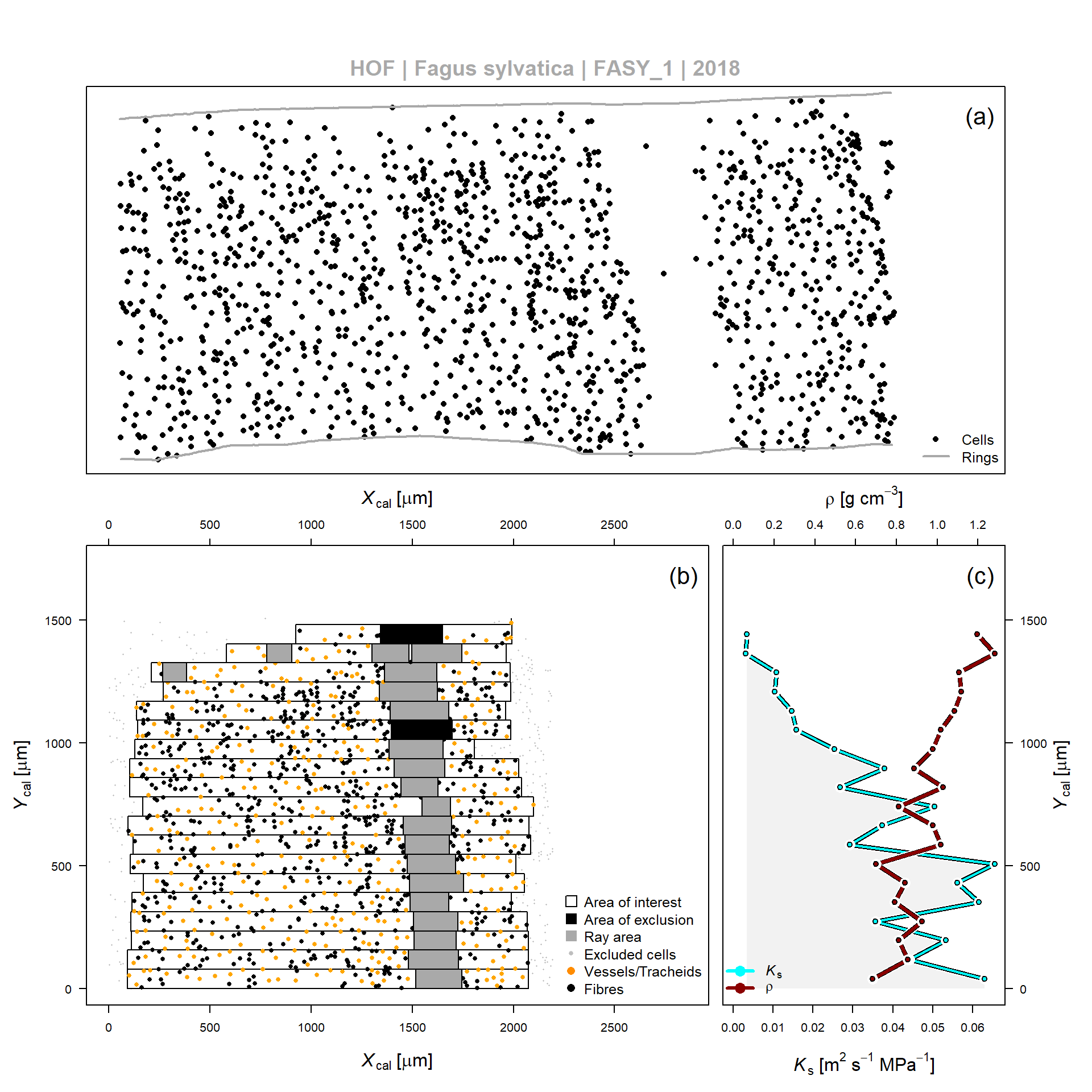
Figure 1: Example of wood anatomical data processing according to SECTOR, for the 2010 tree ring obtained from a Fagus sylvatica tree (FASY_1). (a) Relative center position of vessels and fibers detected by the image analyses software (output from ROXAS). (b) Application of a sectorial binning approach relative to the ring boundary according to the relative position (Ycal and Xcal). Detection algorithms are included which detect rays and areas of exclusion within the bin area (or area of interest). (c) Average theoretical hydraulic conductivity (Ks) and wood density (??) per bin, as defined in (b).
6. SECTOR output
The output of SECTOR is provided in a data.frame format with key wood anatomical parameters.
structure of the output
str(cell_final)
## 'data.frame':	19 obs. of  29 variables:
##  $ site         : Factor w/ 1 level "HOF": 1 1 1 1 1 1 1 1 1 1 ...
##  $ tree         : Factor w/ 1 level "FASY_1": 1 1 1 1 1 1 1 1 1 1 ...
##  $ species      : Factor w/ 1 level "Fagus sylvatica": 1 1 1 1 1 1 1 1 1 1 ...
##  $ sample       : Factor w/ 1 level "HOF": 1 1 1 1 1 1 1 1 1 1 ...
##  $ year         : int  2018 2018 2018 2018 2018 2018 2018 2018 2018 2018 ...
##  $ rw           : num  1512 1512 1512 1512 1512 ...
##  $ area_ray     : num  17776 19412 16295 17054 14916 ...
##  $ area_oi      : num  136826 135190 136766 135910 131517 ...
##  $ area_bin     : num  154602 154602 153061 152964 146433 ...
##  $ area_remove  : num  0 0 0 0 0 0 0 0 0 0 ...
##  $ height_bin   : num  78 78 78 78 78 78 78 78 78 78 ...
##  $ ycal         : num  39 117 195 273 351 429 507 585 663 741 ...
##  $ cwt_param    : num  4 4 4 4 4 4 4 4 4 4 ...
##  $ wood_type    : Factor w/ 1 level "diff": 1 1 1 1 1 1 1 1 1 1 ...
##  $ bin_min      : num  10 10 10 10 10 10 10 10 10 10 ...
##  $ vessel_size  : num  200 200 200 200 200 200 200 200 200 200 ...
##  $ cell_min     : num  15 15 15 15 15 15 15 15 15 15 ...
##  $ cell_max     : num  15000 15000 15000 15000 15000 15000 15000 15000 15000 15000 ...
##  $ ray_min      : num  100 100 100 100 100 100 100 100 100 100 ...
##  $ ray_max      : num  300 300 300 300 300 300 300 300 300 300 ...
##  $ rotate       : num  1 1 1 1 1 1 1 1 1 1 ...
##  $ Kh_sum       : num  9.75e-09 6.84e-09 8.16e-09 5.46e-09 9.02e-09 ...
##  $ Ks           : num  0.0631 0.0442 0.0533 0.0357 0.0616 ...
##  $ LA_sum       : num  84478 66661 70407 58951 69375 ...
##  $ DH           : num  67.7 66.6 69.8 66.5 74.4 ...
##  $ rho          : num  0.682 0.856 0.812 0.924 0.791 ...
##  $ LA_median    : num  17.5 17.7 17.5 17.2 17.9 ...
##  $ add_cells    : num  224 409 403 511 360 379 240 613 575 444 ...
##  $ present_cells: int  63 66 53 55 63 54 56 69 73 64 ...
head(cell_final)
##   site   tree         species sample year       rw area_ray  area_oi area_bin
## 1  HOF FASY_1 Fagus sylvatica    HOF 2018 1512.445 17776.45 136825.6 154602.1
## 2  HOF FASY_1 Fagus sylvatica    HOF 2018 1512.445 19411.68 135190.4 154602.1
## 3  HOF FASY_1 Fagus sylvatica    HOF 2018 1512.445 16294.59 136766.2 153060.7
## 4  HOF FASY_1 Fagus sylvatica    HOF 2018 1512.445 17054.05 135910.2 152964.2
## 5  HOF FASY_1 Fagus sylvatica    HOF 2018 1512.445 14915.98 131516.6 146432.6
## 6  HOF FASY_1 Fagus sylvatica    HOF 2018 1512.445 20773.32 126268.0 147041.3
##   area_remove height_bin ycal cwt_param wood_type bin_min vessel_size cell_min
## 1           0         78   39         4      diff      10         200       15
## 2           0         78  117         4      diff      10         200       15
## 3           0         78  195         4      diff      10         200       15
## 4           0         78  273         4      diff      10         200       15
## 5           0         78  351         4      diff      10         200       15
## 6           0         78  429         4      diff      10         200       15
##   cell_max ray_min ray_max rotate       Kh_sum         Ks   LA_sum       DH
## 1    15000     100     300      1 9.753501e-09 0.06308778 84478.38 67.71871
## 2    15000     100     300      1 6.840237e-09 0.04424415 66661.38 66.64492
## 3    15000     100     300      1 8.163268e-09 0.05333352 70406.69 69.83946
## 4    15000     100     300      1 5.457113e-09 0.03567575 58950.61 66.52932
## 5    15000     100     300      1 9.015987e-09 0.06157089 69374.98 74.43297
## 6    15000     100     300      1 8.270567e-09 0.05624655 64862.34 72.55115
##         rho LA_median add_cells present_cells
## 1 0.6821773    17.470       224            63
## 2 0.8555047    17.655       409            66
## 3 0.8121723    17.470       403            53
## 4 0.9243761    17.200       511            55
## 5 0.7914541    17.890       360            63
## 6 0.8405609    17.140       379            54
Besides the descriptive columns (i.e., site, tree, species, and sample), we provide for each year (year) the annual ring width (rw in micron).
Moreover, the data.frame includes in square micron the detected ray area (area_ray), area of interest per bin (area_oi), the bin area (area_bin) and the area not assigned to rays or cells (area_remove),
next to the height of each bin in micron (height_bin) and the center of the bin in the radial direction (ycal).
All used parameters are stored in the columns, cwt_param, wood_type, bin_min, vessel_size, cell_min, cell_max, ray_min, ray_max and rotate.
The following relevant wood anatomical outputs are provided per bin (or sector):
Kh_sum: Theoretical hydraulic conductivity ($ m^4 s^{-1} MPa^{-1} $) as approximated by Poiseuille’s law and adjusted to elliptical tubes. The calculation for Kh comes from Nonweiler TRF. 1975. Flow of biological fluids through non-ideal capillaries. In: Zimmermann MH, Milburn JA (eds) Encyclopaedia of plant physiology, new series, vol 1. Transport in plants. I. Phloem transport, Appendix I. Springer, Berlin Heidelberg New York, pp 474-477.Ks: Theoretical xylem-specific hydraulic conductivity for a bin ($ m^2 s^{-1} MPa^{-1} $) assuming a tube length of $ 1 m $: Kh/(bin area-area of exclusion; in $ m^2 $).DH: Hydraulic diameter of cell (i.e. correcting for effect of elliptical shape on flow; in microns); see Lewis AM, Boose ER. 1995. Estimating Volume Flow Rates Through Xylem Conduits. American Journal of Botany 82: 1112-1116.rho: Overall mean relative anatomical cell density (in $ g~cm^{-3}$ ). Assuming a fixed density of wall material of $ 1.504~g~cm^{-3} $ as found by Kellogg RM, Wangaard FF (1969) Variation in the cell-wall density of wood. Wood and Fiber Science 1:180-204. ATTENTION: may include artefacts from pit-pore associated widening.LA_median: Median lumen area of all detected cell within a bin.add_cells: Added cells within the bin due to the presence of empty space not assigned to rays or detected as an area of exclusion.present_cells: Detected cells within the bin area.
For more information on how these parameters are calculated, one can have a look at the ROXAS user manual (https://www.wsl.ch/en/forest/tree-ring-research/products/roxas.html).
Richard L. Peters
Post-doc
My research interests include tree physiology, wood anatomy and mechanistic modelling.