CLIMCOR Workflow

1. Background

This tutorial is about systematically screening different season lengths when performing climate-growth relationship analyses on tree-ring width measurements. Trees do not care about months or seasons as we define them. Therefore, it is essential to check all possible season lengths and ending months.

Because we like working with the time-series class (ts()) we need to change the class() of all R objects (tree-ring and climate data) to that of a time series. Additionally we need some custom-built functions to detrend.

2. Set-up steps

First, we need to load some required libraries that the code is based on.

#install package if necessary
packages <- c("dplR","MASS","dyn","lattice","latticeExtra","zoo","pspline")
try(install.packages(setdiff(packages, rownames(installed.packages()))))
library(dplR)
library(MASS)
library(dyn)
library(lattice)
library(latticeExtra)
library(zoo)
library(pspline)

3. Import data

Below one will load an example tree-ring series and climate data.

#load tree-ring data
TRW<-read.rwl("https://raw.githubusercontent.com/deep-org/materials/main/data/general_statistics/01_climate_cor_trw/saviese.txt")
## Attempting to automatically detect format.
## Assuming a Tucson format file.
## There does not appear to be a header in the rwl file
## There are 32 series
## 1    	10S01A  	 1921	 2005	0.01
## 2    	10S01B  	 1926	 2005	0.01
## 3    	10S03A  	 1928	 2005	0.01
## 4    	10S03B  	 1920	 2005	0.01
## 5    	10S04A  	 1924	 2005	0.01
## 6    	10S04B  	 1924	 2005	0.01
## 7    	10S05A  	 1931	 2005	0.01
## 8    	10S05B  	 1928	 2005	0.01
## 9    	10S08A  	 1923	 2005	0.01
## 10   	10S08B  	 1924	 2001	0.01
## 11   	10S20A  	 1924	 2005	0.01
## 12   	10S20B  	 1926	 2005	0.01
## 13   	10S21A  	 1926	 2005	0.01
## 14   	10S21B  	 1926	 2005	0.01
## 15   	10S22A  	 1926	 2005	0.01
## 16   	10S22B  	 1926	 2005	0.01
## 17   	10S23A  	 1926	 2005	0.01
## 18   	10S23B  	 1926	 2005	0.01
## 19   	10S24A  	 1925	 2005	0.01
## 20   	10S24B  	 1924	 2005	0.01
## 21   	10S25A  	 1893	 2005	0.01
## 22   	10S25B  	 1887	 2005	0.01
## 23   	10S26B  	 1943	 2005	0.01
## 24   	10S28A  	 1820	 2005	0.01
## 25   	10S28B  	 1819	 2005	0.01
## 26   	10S29A  	 1902	 2005	0.01
## 27   	10S50A  	 1872	 2005	0.01
## 28   	10S50B  	 1894	 2005	0.01
## 29   	10S51A  	 1887	 2005	0.01
## 30   	10S51B  	 1898	 2005	0.01
## 31   	10S57A  	 1841	 2005	0.01
## 32   	10S58A  	 1872	 2005	0.01

#apply detrending
TRW<-detrend(TRW,method="Spline",nyrs=50)

#transform the data.frame to a time series object starting in the first year of the original data.frame
TRW<-ts(apply(TRW,1,tbrm),start=as.numeric(rownames(TRW))[1])

The first climate data we will work with are precipitation time series from the E-OBS dataset, you can download from the KNMI climate explorer.

#loading climate data in the CRU format with 13 columns (1= year, 2:13= months)
climate<-read.table("https://raw.githubusercontent.com/deep-org/materials/main/data/general_statistics/01_climate_cor_trw/precip.txt",header=F)
climate[climate==-999.9]<-NA #transform -999.9 to NAs

Note, E-OBS reports mean daily precipitation per month, so the values have to be multiplied by the number of days per month. With CRU and most other products, this step can be skipped.

#correct for leap years for February (%%4==0 means: which year divided by 4 has the rest = 0, i.e. the module of division by 4 equaling 0)
month.length<-c(31,28,31,30,31,30,31,31,30,31,30,31)
for(i in 2:13){
  if(i==3){
    climate[,3]<-climate[,3]*(28+1*(climate[,1]%%4==0))
  }else{
    climate[,i]<-climate[,i]*month.length[i-1]
  }
}

4. Data and function preparation

Next, we want to aggregate the monthly climate data to seasons of differing lengths. Maximum season length is by default set to 12 months. The function should work on longer time scales but is currently not tested beyond 12 months. Consider including `lag=2 into runningclimate function.

#load required functions
runningclimate_new<-function(climate,stat=c("mean","sum"),max.length=12){
  x.ts<-ts(climate[,2:13],start=climate[1,1]) #transform CRU style climate data into time-series format
  x.lag<-stats::lag(x.ts,k=-1) #create lag1 series
  x1<-ts.union(x.lag,x.ts) #combine lagged and original series
  max.length<-max.length  #default to 12 months
  stat<-stat #no default is given
  seasons<-rep(list(x1),max.length)
  for(i in 2:max.length){
    seasons[[i]]<-ts(cbind(matrix(rep(rep(NA,nrow(x1)),i-1),ncol=i-1),t(rollapply(t(seasons[[i]]),i,stat,na.rm=T,align='right'))),start=climate[1,1])
    colnames(seasons[[i]])<-c(paste0("p",month.abb),month.abb) }
  output<-seasons
}

Climatesite<-runningclimate_new(climate,stat="sum") #use "sum" when working with precipitation, use "mean" when working temperature

This next function fits cubic smoothing splines to a ts-class object and is needed for the other two functions below. Courtesy of David C. Frank.

#load required functions
spline.det <- function(x,smoothing) {
require(pspline)
  spline.p.for.smooth.Pspline<-function(year)  {
    p <- .5/((6*(cos(2*pi/year)-1)^2/(cos(2*pi/year)+2)))
    return(p)
  }
   fy <- function(object) {
    fyos<- function(x) {
      L <- !is.na(x)
      idx <- c(NA, which(L))[cumsum(L) + 1]
      fy <- min(idx,na.rm=TRUE)
      return(fy)
    }

    ifelse (is.mts(object),
            rel.years <- apply(object,2,fyos),
            rel.years <- fyos(object))

    calyears <- rel.years+start(object)[1]-1
    return(calyears)
  }

  ly <- function(object) {

    fyos<- function(x) {
      L <- !is.na(x)
      idx <- c(NA, which(L))[cumsum(L) + 1]
      fy <- max(idx,na.rm=TRUE)
    }

    ifelse (is.mts(object),
            rel.years <- apply(object,2,fyos),
            rel.years <- fyos(object))

    calyears <- rel.years+start(object)[1]-1
    return(calyears)
  }

  ifelse ((is.null(ncol(x))),x2 <- ts.union(x,x), x2 <- x)
  fyarray <- start(x2)[1]
  lyarray <- end(x2)[1]
  begin <- fy(x2)
  end <- ly(x2)
  smoothedarray <- x2

  spline.p <- spline.p.for.smooth.Pspline(smoothing)

  for (i in 1:ncol(x2)) {
    temp <- smooth.Pspline((begin[i]:end[i]),x2[(begin[i]-fyarray+1):(end[i]-fyarray+1),i],spar=spline.p,method=1)
    smoothedarray[(begin[i]-fyarray+1):(end[i]-fyarray+1),i]  <- temp$ysmth
  }

  if (is.null(ncol(x))) {smoothedarray <- smoothedarray[,-1]}
  residualarray <- x-smoothedarray
  ratioarray <- x/smoothedarray

  output <- list(x=x,smoothedarray=smoothedarray,residualarray=residualarray,ratioarray=ratioarray)
  return(output)
}

The function automatically returns four objects. 1) The original time series, 2) the smoothing function, 3) the residual array (x-smoothing), and 4) the ratio array (x/smoothing). For climate data (especially temperature) we need the residual array of that detrending.

Next up is the systematic correlation of the tree-ring chronology against all aggregated climate series. The output graph is similar to the output of the R package SPEI ( Beguería & Vicente-Serrano, 2017) and the CLIMTREG program ( Beck et al., 2013).

#load required functions
Climateplot_new<-function(TRW,Climatesite,fyr=tsp((Climatesite[[1]]))[1],lyr=tsp((Climatesite[[1]]))[2],detrended=c("Yes","No"),spline.length){   ####Climatesite=your climate data run through runningclimate_new(),TRW=Tree ring chronology with time series class,fyr=first year, lyr=last year
  climatecor<-NULL

  if(detrended=="Yes"){
    tsstart<-tsp((Climatesite[[1]]))[1]
    for (i in 1:length(Climatesite)){
      Climatesite[[i]]<-ts(apply(Climatesite[[i]],2,function(x)if(sum(complete.cases(x))>3){spline.det(ts(x),spline.length)$residualarray}else{rep(NA,length(x))}),start=tsstart)
      climatecor[[i]]<-cor(ts.union(Climatesite[[i]],window(TRW,fyr,lyr)),use="p")
    }
    levelplotmatrix<-matrix(NA,length(Climatesite),22)
    for (i in 1:length(Climatesite)){
      levelplotmatrix[i,]<-climatecor[[i]][1:22,25]
    }
  }else{
    for (i in 1:length(Climatesite)){
      climatecor[[i]]<-cor(ts.union(Climatesite[[i]],window(TRW,fyr,lyr)),use="p")
    }
    levelplotmatrix<-matrix(NA,length(Climatesite),22)
    for (i in 1:length(Climatesite)){
      levelplotmatrix[i,]<-climatecor[[i]][1:22,25]
    }
  }
  rownames(levelplotmatrix)<-names(1:length(Climatesite))
  colnames(levelplotmatrix)<-c(paste0("p",month.abb),month.abb[1:10])
  return(levelplotmatrix)
}

5. Climate correlations

If your chronology is spline-detrended, you should spline-detrend the climate data as well. Splines remove a fixed amount of variance at a given frequency. Keeping those lower frequencies (and trends) in the climate data while removing them from tree-ring data will likely yield distorted correlation coefficients. Thus, we strongly recommend using the same spline stiffness for both the climate and tree-ring data.

#generating the correlation plots
silly_cor<-Climateplot_new(TRW,Climatesite,1950,2005,"Yes",50)
P1<-contourplot(t(silly_cor),region=T,contour=F,lwd=0.4,col.regions=colorRampPalette(c("red","yellow","white","green3","blue")),at=c(seq(-0.825,0.825,0.05)),xlab="Months",ylab="Window length")
P2<-contourplot(t(silly_cor),labels=T,col.regions=F,region=F,lwd=0.4,at=c(seq(-0.80,0.80,0.05)))
PP<-P1+P2
print(PP)

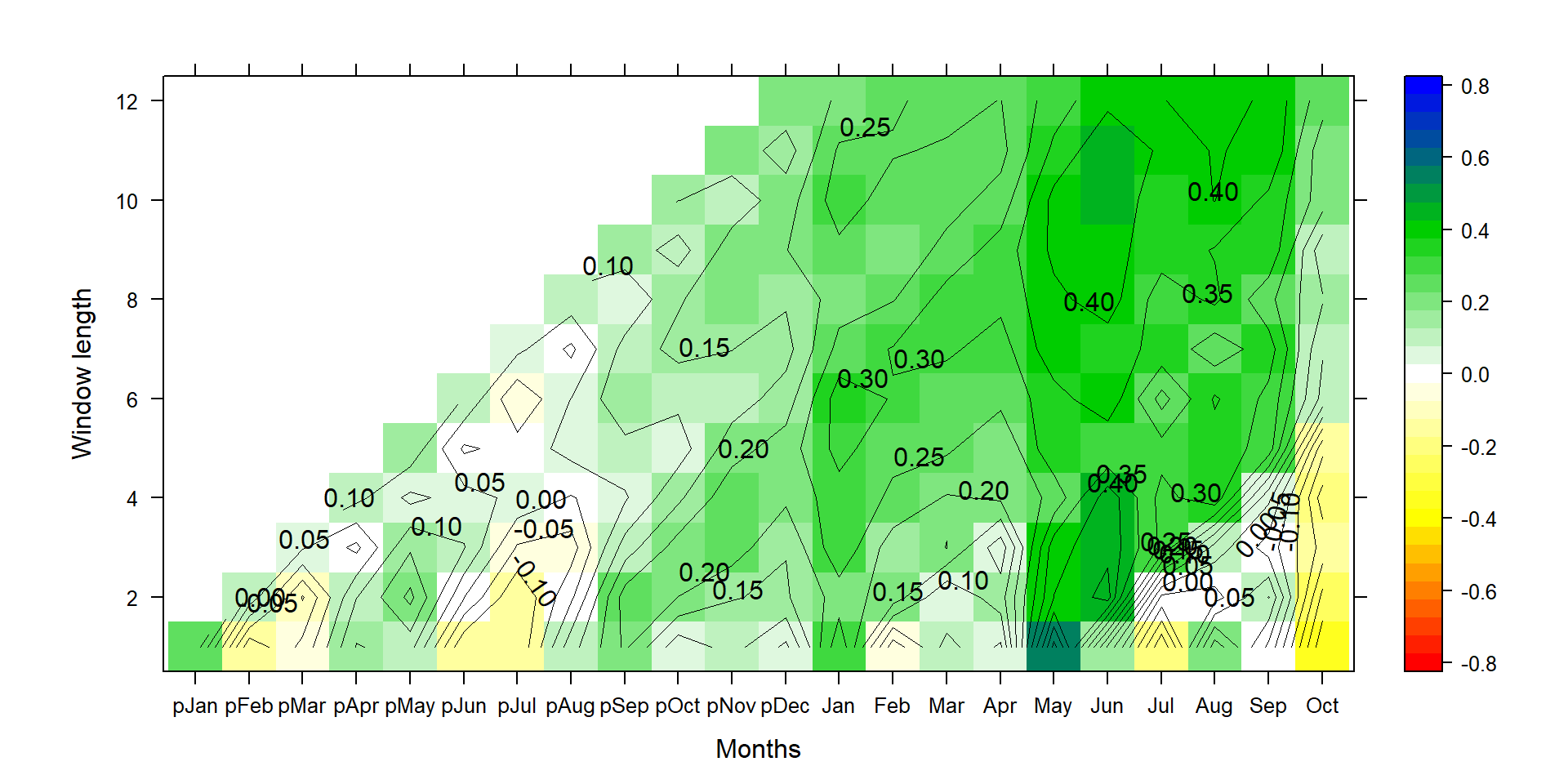
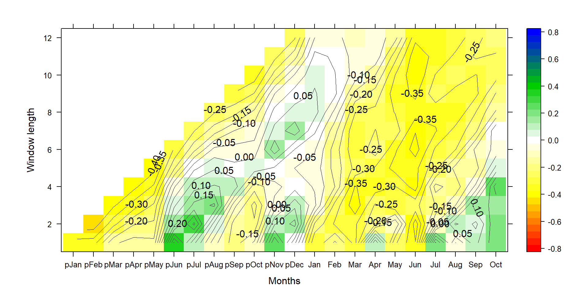
Figure 1: This graph shows climate-growth correlations for different end months (along the x-axis) and different season lengths (y-axis). Positive correlations are shown in green and blue, and negative correlations in yellow to redish colors.

Combining P1 and P2 allows for more flexibility for the plotting. One could add a third layer, specifying a certain threshold value, i.e. where p<0.01 via specifying that threshold (e.g., at=0.3) and increasing line width (e.g., lwd=1).

Correlation is the standardized regression coefficient, where both standard deviations of the tree-ring data and the climate data are set to 1. The correct interpretation is thus primarily noise-related. A high (absolute) correlation coefficient means there is little noise in a relationship. But it doesn’t allow users to draw conclusions on the actual magnitude of impact on radial tree growth. This is especially true, when one wants to compare climate impacts at two different sites, or for two species growing at the same site. Correlation is not directly related to climate sensitivity, at least not on its own. It’s only the fraction of signal explained.

To quantify actual climate impact, we need the unstandardized regression coefficient. In the example with precipitation, we multiply by 100, to return a relative growth change in response to a 100mm change in precipitation in the respective season (a bit more realistic than retrieving the impact for 1mm precipitation change).

First, the function:

#load required functions
Climateslopeplot_new<-function(TRW,Climatesite,fyr=tsp((Climatesite[[1]]))[1],lyr=tsp((Climatesite[[1]]))[2],detrended=c("Yes","No"),spline.length,weighted=TRUE){ #Climatesite=your climate data, TRW=Tree-ring chronology, fyr=first year, lyr=last year
   climatecor<-matrix(NA,nrow=length(Climatesite),ncol=22)
  if(detrended=="Yes"){
    tsstart<-tsp(Climatesite[[1]])[1]
    for (i in 1:length(Climatesite)){
      Climatesite[[i]]<-ts(apply(Climatesite[[i]],2,function(x)if(sum(complete.cases(x))>3){spline.det(ts(x),spline.length)$residualarray}else{rep(NA,length(x))}),start=tsstart)
      for(k in 1:22){
        if(sum(complete.cases(Climatesite[[i]][,k]))>3){
          if(weighted==T){
            w<-rlm(window(TRW,fyr,lyr)~window(Climatesite[[i]][,k],fyr,lyr))$w
            if(k<=12){
              climatecor[i,k]<-coef(dyn$lm(window(TRW,fyr+1,lyr)~window(Climatesite[[i]][,k],fyr+1,lyr),weights=w))[2]
            }else{
              climatecor[i,k]<-coef(dyn$lm(window(TRW,fyr,lyr)~window(Climatesite[[i]][,k],fyr,lyr),weights=w))[2]
            }
          }else{
            climatecor[i,k]<-coef(dyn$lm(window(TRW,fyr,lyr)~window(Climatesite[[i]][,k],fyr,lyr)))[2]
          }
        }else{
          next
        }
      }
    }
    levelplotmatrix<-climatecor
  }else{
    for (i in 1:length(Climatesite)){
      for(k in 1:22){
        if(sum(complete.cases(Climatesite[[i]][,k]))>3){
          if(weighted==T){
            w<-rlm(window(TRW,fyr,lyr)~window(Climatesite[[i]][,k],fyr,lyr))$w
            if(k<=12){
              climatecor[i,k]<-coef(dyn$lm(window(TRW,fyr+1,lyr)~window(Climatesite[[i]][,k],fyr+1,lyr),weights=w))[2]
            }else{
              climatecor[i,k]<-coef(dyn$lm(window(TRW,fyr,lyr)~window(Climatesite[[i]][,k],fyr,lyr),weights=w))[2]
            }
          }else{
            climatecor[i,k]<-coef(lm(window(TRW,fyr,lyr)~window(Climatesite[[i]][,k],fyr,lyr)))[2]
          }
        }else{
          next
        }}}
    levelplotmatrix<-climatecor
  }
  rownames(levelplotmatrix)<-names(1:12)
  colnames(levelplotmatrix)<-c(paste0("p",month.abb),month.abb[1:10])
  return(levelplotmatrix)
}

You can choose between ordinary least square regression, or the robust linear regression that down-weights outliers.

#generating the new contourplot
silly_slope<-Climateslopeplot_new(TRW,Climatesite,1950,2005,"Yes",50,weighted=F)
P1<-contourplot(t(silly_slope*100),region=T,contour=F,lwd=0.4,col.regions=colorRampPalette(c("red","yellow","white","green3","blue")),at=c(seq(-0.305,0.305,0.01)),xlab="Months",ylab="Window length")
P2<-contourplot(t(silly_slope*100),labels=T,col.regions=F,region=F,lwd=0.4,at=c(seq(-0.30,0.30,0.01)))
PP<-P1+P2
print(PP)

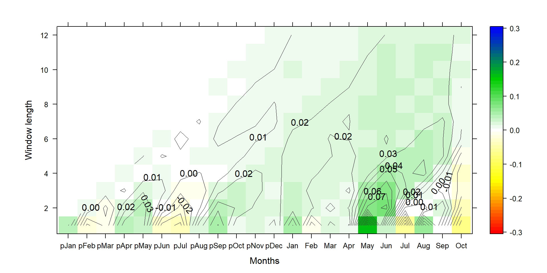
Because we sum up individual months, the comparison is actually a bit unfair and biased towards yielding strongest impacts on short season lengths. The standard deviation of the annual time series (aggregated over 12 months) is ~6 times higher than at monthly periods, so 100 mm change at annual scale is not really a lot, while it is more than a standard deviation on the monthly scale.

#standard deviation of May precipitation
sd(Climatesite[[1]][,17],na.rm=T)
## [1] 44.72265

#standard deviation of Mar-Jun precipitation
sd(Climatesite[[4]][,18],na.rm=T)
## [1] 121.7759

#standard deviation of pSep-Aug precipation
sd(Climatesite[[12]][,20],na.rm=T)
## [1] 275.4319

#generating the new contourplot
P1<-contourplot(t(silly_slope*c(1:12)*100),region=T,contour=F,lwd=0.4,col.regions=colorRampPalette(c("red","yellow","white","green3","blue")),at=c(seq(-0.425,0.425,0.05)),xlab="Months",ylab="Window length")
P2<-contourplot(t(silly_slope*c(1:12)*100),labels=T,col.regions=F,region=F,lwd=0.4,at=c(seq(-0.40,0.40,0.05)))
PP<-P1+P2
print(PP)

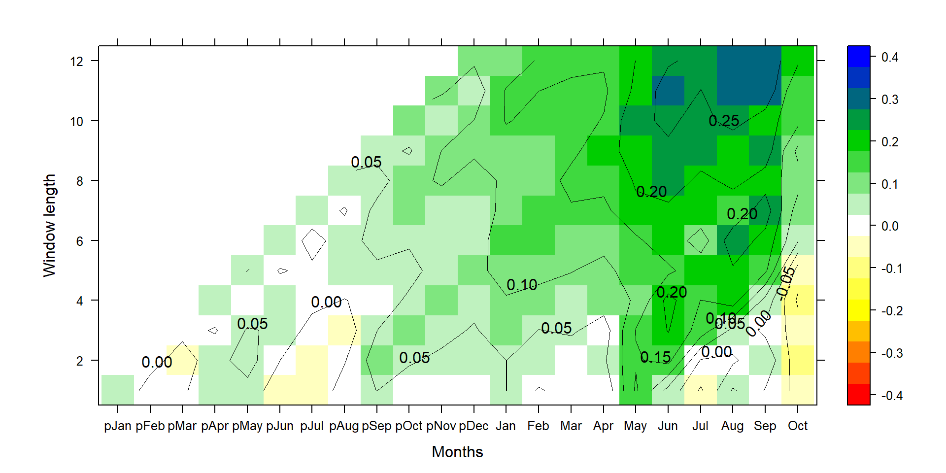
This yields very similar results compared to the aggregation via stat="mean" instead of stat="sum" and shows the results if every month in that season had 100 mm more precipitation. This nicely shows the effect of using sum or mean for precipitation aggregation and the derivation of regression coefficients.

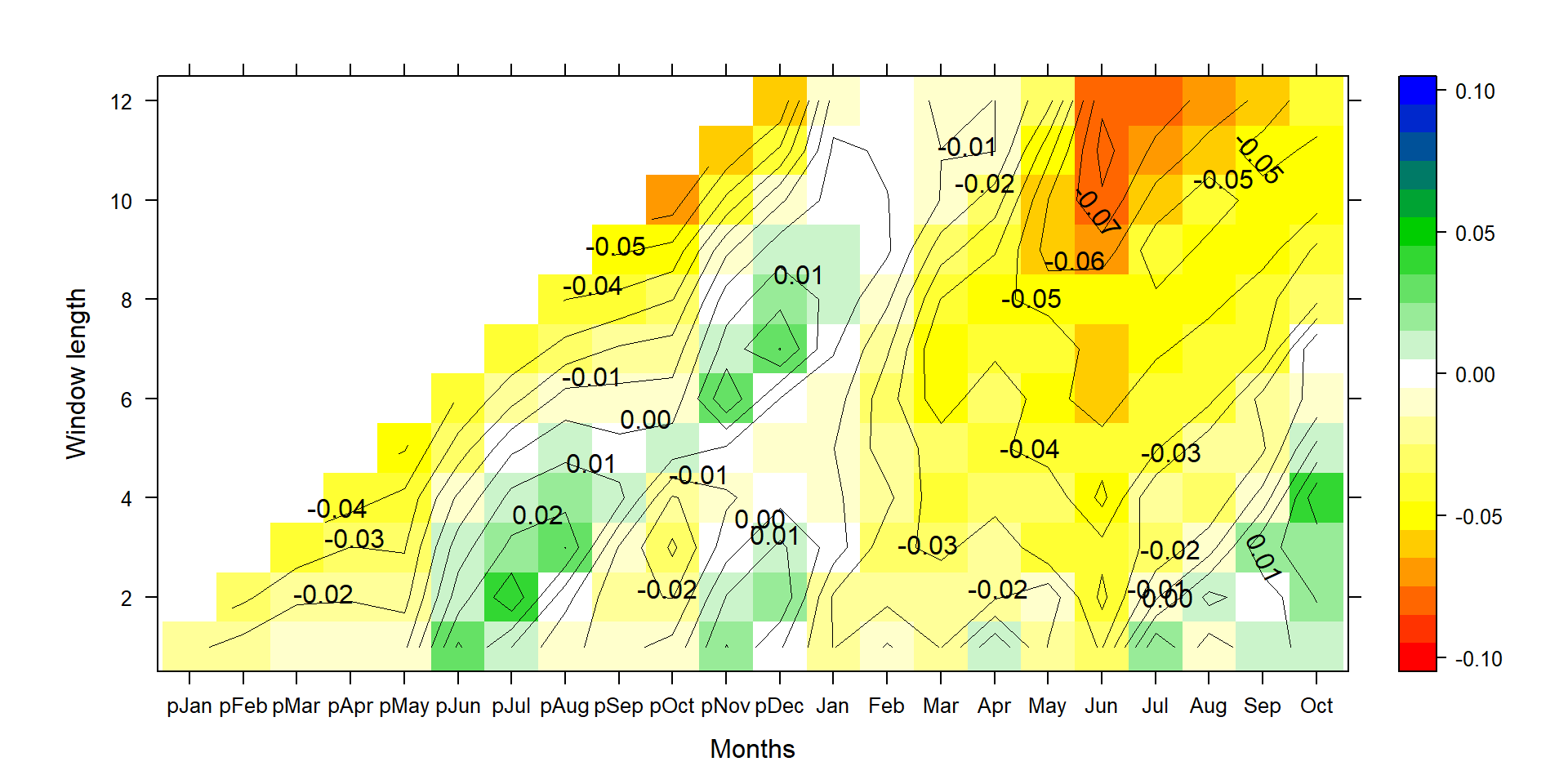
Now let’s see what happens when we normalize each climate time series by its standard deviation.

#compute standard deviation per aggregation size ( sapply() ) and per each column in each aggregation step (function(x)apply(x,2,sd))
climate_sd<-sapply(Climatesite,function(x)apply(window(x,1950,2005),2,sd,na.rm=T))
P1<-contourplot(t(silly_slope*t(climate_sd)[,1:22]),region=T,contour=F,lwd=0.4,col.regions=colorRampPalette(c("red","yellow","white","green3","blue")),at=c(seq(-0.105,0.105,0.01)),xlab="Months",ylab="Window length")
P2<-contourplot(t(silly_slope*t(climate_sd)[,1:22]),labels=T,col.regions=F,region=F,lwd=0.4,at=c(seq(-0.10,0.10,0.01)))
PP<-P1+P2
print(PP)

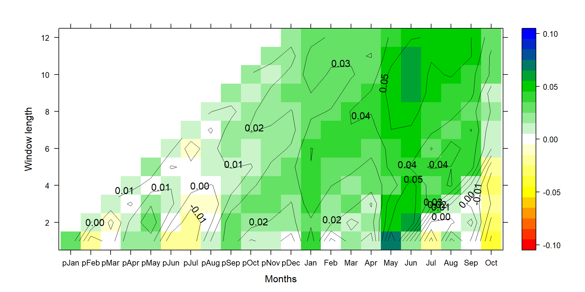
The graph looks pretty similar in its pattern to the correlation graph from above. But now we know how much relative growth change a standard deviation change in the respective climate time series invokes.

Let’s have a look at the same analysis using temperature data.

#upload temperature data
climate<-read.table("https://raw.githubusercontent.com/deep-org/materials/main/data/general_statistics/01_climate_cor_trw/tmean.txt",header=F)
climate[climate==-999.9]<-NA #transform -999.9 to NAs

#perform the analysis
Climatesite<-runningclimate_new(climate,stat="mean")
silly_cor<-Climateplot_new(TRW,Climatesite,1950,2005,"Yes",50)
P1<-contourplot(t(silly_cor),region=T,contour=F,lwd=0.4,col.regions=colorRampPalette(c("red","yellow","white","green3","blue")),at=c(seq(-0.825,0.825,0.05)),xlab="Months",ylab="Window length")
P2<-contourplot(t(silly_cor),labels=T,col.regions=F,region=F,lwd=0.4,at=c(seq(-0.80,0.80,0.05)))
PP<-P1+P2
print(PP)

silly_slope<-Climateslopeplot_new(TRW,Climatesite,1950,2005,"Yes",50,weighted=F)
P1<-contourplot(t(silly_slope),region=T,contour=F,lwd=0.4,col.regions=colorRampPalette(c("red","yellow","white","green3","blue")),at=c(seq(-0.105,0.105,0.01)),xlab="Months",ylab="Window length",main=title)
P2<-contourplot(t(silly_slope),labels=T,col.regions=F,region=F,lwd=0.4,at=c(seq(-0.10,0.10,0.01)))
PP<-P1+P2
print(PP)

This graph shows how much the relative tree growth changes for a 1°C increase in mean temperature (0.07=7%).

#perform the analysis
climate_sd<-sapply(Climatesite,function(x)apply(x,2,sd,na.rm=T))
P1<-contourplot(t(silly_slope*t(climate_sd)[,1:22]),region=T,contour=F,lwd=0.4,col.regions=colorRampPalette(c("red","yellow","white","green3","blue")),at=c(seq(-0.105,0.105,0.01)),xlab="Months",ylab="Window length",main=title)
P2<-contourplot(t(silly_slope*t(climate_sd)[,1:22]),labels=T,col.regions=F,region=F,lwd=0.4,at=c(seq(-0.10,0.10,0.01)))
PP<-P1+P2
print(PP)

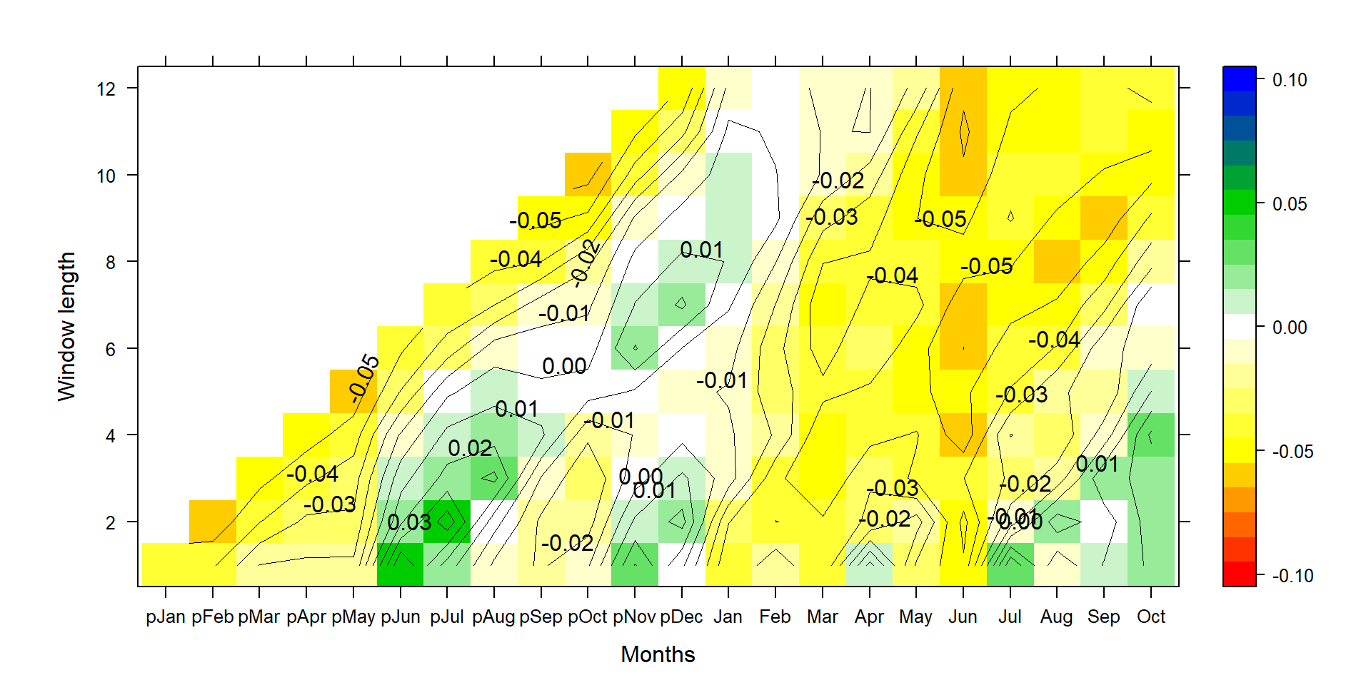
Again, this graph shows the same pattern as in the correlation plot, but for normalized climate data and the un-normalized ring-width index, a percentage tree growth change per standard deviation change in temperature.

6. Some afterthoughts

The R package dendroTools from Jevšenak and Levanič (2018) does something very similar but uses daily climate data.