datacleanr Workflow

1. Background

Here we introduce datacleanr, a recently developed app. It is a flexible and efficient tool for interactive data cleaning, and is inherently interoperable, as it seamlessly integrates into reproducible data analyses pipelines in R. It can deal with nested tabular, as well as spatial and time series data. We present how to use the app and show two use-cases - one for processing wood anatomical data and one for environmental data (soil respiration - \(CO_2\) flux). Detailed documentation and animated examples for each feature can be found at the-hull.github.io/datacleanr.

2. Installation

The latest release on CRAN can be installed using:

# also installing dplyr for later use
packages <- (c("datacleanr", "RAPTOR", "dplyr", "forcats"))
install.packages(setdiff(packages,
                         rownames(installed.packages())))

library(datacleanr)
library(dplyr)

You can install the development version of datacleanr with:

packages <- (c("remotes"))
install.packages(setdiff(packages,
                         rownames(installed.packages())))

remotes::install_github("the-hull/datacleanr")

3. Design and features

datacleanr is developed using the shiny package, and relies on informative summaries, visual cues and interactive data selection and annotation. All data-altering operations are documented, and converted to valid R code (reproducible recipe), that can be copied, sent to an active RStudio script, or saved to disk.

The documentation for the app (?dcr_app()) explains the basic use and all features. Throughout the app, there are conveniently-placed help links that provide details on features.

There are four tabs in the app for these tasks:

• Set-up & Overview: define nesting structure based on (multiple) groups.
• Filtering: use R expression to filter/subset data.
• Visual Cleaning and Annotating: generate bivarirate (time series) plots and maps, as well as highlight and annotate individual observations. Cycle through nested groups to expedite exploration and cleaning. Histograms of original vs. ‘cleaned’ data can be generated.
• Extract: generate reproducible recipe and define outputs. dcr_app also returns all intermediate and final outputs invisibly to the active R session for later use (e.g. when batch processing)

Note, maps require columns lon and lat (X and Y) in decimal degrees in the data set to render.

4. Additional features

• Grouping: the grouping defined in the “Set-up and Overview” tab is carried forward through the app. These groups can be used to cycle through nested/granular data, and considerably speed up exploration and cleaning. These groups are also available for filtering (Filtering tab), where filter expressions can be scoped to group level (i.e. no groups, individual, all groups).
• Interoperability: when a logical (TRUE\FALSE) column named .dcrflag is present, corresponding observations are rendered with different symbols in plots and maps. Use this feature to validate or cross-check external quality control or outlier flagging methods.
• Batching: If data sets are too large, or too deeply nested (e.g. individual, plot, site, region, etc.), we recommend a split-combine approach to expedite the processing.

iris_split <- split(iris, iris$Species)

output <- lapply(iris_split,
       dcr_app)

5. datacleanr with Wood Anatomical Measurements

RAPTOR is a powerful tool to assimilate and generate cell-level measurements of coniferous, woody plants generated by ROXAS. It will serve as the basis to generate a dataset, which we will subsequently clean. More details on RAPTOR can be found in Peters et al. (2018) and in the dedicated DEEP tutorial here.

In the following, we generate a spatially-explicit representation of tracheids by identifying individual radial files (a “row” of cells produced from the same cambial mother). This is done through two complex “cell search” algorithms, to detect the first (early-wood) cell formed in a year with first.cells(), and then starting from these, determining which subsequent cells form a row with the function pos.det(). These algorithms assume a vertical (bottom to top) growth on a plane, and therefore some rings / samples need to be rotated (aligned()) first.

library(RAPTOR)

# grab example data
input <- is.raptor(example.data(species = "MOUNT_PINUS"),
                   str = FALSE)
# rotate annual rings where necessary
# so that detection algorithms can operate seamlessly
aligned <- align(input,
                 list = c("h", "h", "h", 0.03),
                 make.plot = FALSE)

# identify first cell in every annual ring
first <- first.cell(aligned,
                    frac.small = 0.2,
                    yrs = FALSE,
                    make.plot = FALSE)

# identify all cells along radial files (ROWs),
# starting from first cells
output <- pos.det(first,
  swe = 0.7, sle = 3, ec = 1.75, swl = 0.5, sll = 5, lc = 10,
  prof.co = 1.7, max.cells = 0.7, yrs = FALSE, aligning = FALSE, make.plot = TRUE
)

The output can be used directly in datacleanr, but a few additional steps make the subsequent processing considerably more efficient. Through RAPTOR's alignment process, all rings are assumed to originate on a planar coordinate system at (0,0), causing overlap during plotting. We will space out annual rings, and add factors for grouping, which will be used to visualize years and rows individually.

# grab maximum YCAL location and add a buffer for convenience
# this is used to space out rings below
buffer <- 100
max_ring_size <- output %>%
  group_by(YEAR) %>%
  summarize(max_length = max(YCAL, na.rm = TRUE) + buffer) %>%
  mutate(cumulative_year_length = cumsum(max_length))

output_dcr <- output %>%
  left_join(max_ring_size) %>%
  mutate(YEAR_dcr = as.factor(YEAR),
         # leverage RAPTOR's row identification
         ROW_dcr = as.factor(ifelse(is.na(ROW), "0",ROW )) %>%
           forcats::fct_reorder(as.numeric(as.character(.))),
         # space out overlapping rings
         YCAL_dcr =  YCAL + cumulative_year_length)

datacleanr::dcr_app(output_dcr)

We can now use these adjustment to expedite the interactive processing once the app is launched:

1. Set YEAR_dcr and ROW_dcr as the grouping variables on the app’s first tab (Set-up & Overview)
2. On the Visual Cleaning & Annotating tab, set XCAL, YCAL_dcr and CA (Cell Area) for the X Y and Z var, respectively, and click Plot.
3. Use the grouping table on the left to hide / show entire years and rows of interest. For example, type 2007 in the search box, and highlight all table rows, followed by a click on (Update). Use a SHIFT / CMD + Click on the first and last rows to highlight everything in between in one go.
4. In the grouping table, row’s with a ROW_dcr value of 0 include all cells that RAPTOR could not assign to a continuous, radial file. You can toggle these on and off by selecting the corresponding legend item (`1) to the right (rather than updating the plotting groups on the left).
5. Some rows are conspicuous, and should/could be checked in ROXAS, as well as in RAPTOR outputs - adjusting search window sizes in pos.det() may aid here. Alternatively, given the wealth of other available rows for subsequent analyses, some problematic rows can be excluded.
6. One such that requires additional scrutiny is represented by legend item 31 (ROW_dcr = 30) - the spacing of the first three cells appears too large.
7. On the lower left side of the tab, give an appropriate label for an annotation, click Auto-annotate and use the lasso tool to highlight the conspicuous ROW.
8. Navigate to the Extract tab, and either send your recipe back to RStudio, or copy it to your clipboard.
9. Close the app.

Figure 1: datacleanr‘s Visual Cleaning and Annotating tab after following steps 1-7 above. Note the orange boxes highlighting the selected outliers, and their respective annotation, while the green boxes highlight the non-assigned cells (customly defined into’ROW_dcr 0’) in the grouping table and figure legend.

The workflow (above steps 1-7) allows rapidly checking and quality-controlling RAPTORs results, which can either inform repeated cell-searching and position detection, or be the basis for additional cleaning (i.e., removing observations). datacleanr is hence a powerful tool to facilitate the generation of high-quality wood anatomical datasets, which can subsequently be linked to other environmental data.

6. datacleanr with Environmental Data: Soil Respiration Example

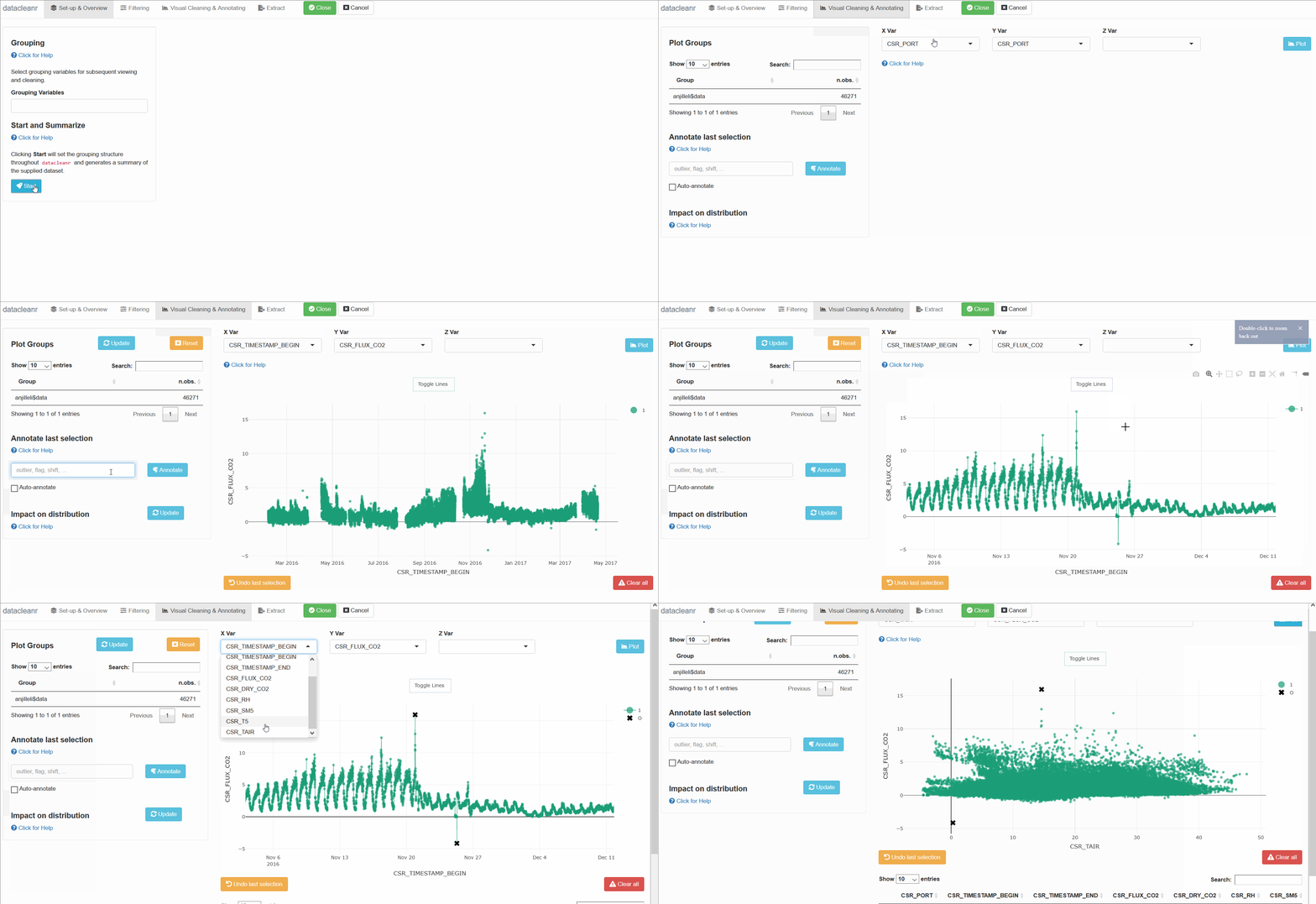
COSORE is a community-driven soil respiration database, recently introduced with a manuscript published here by Bond-Lamberty et al.. The database provides soil respiration flux estimates, as well as meta data across multiple data sets.

The following two examples show the use of grouping tables as well as rapid generation of multiple visualizations to quality control data across a datasets dimensions, as in the example below.

remotes::install_github("bpbond/cosore")
library(dplyr)

# check data base info
db_info <- cosore::csr_database()
tibble::glimpse(db_info)

# grab one data set and explore in detail
dset <- "d20190409_ANJILELI"
anjilleli <- cosore::csr_dataset(dset)
tibble::glimpse(anjilleli$description)


datacleanr::dcr_app(anjilleli$data)

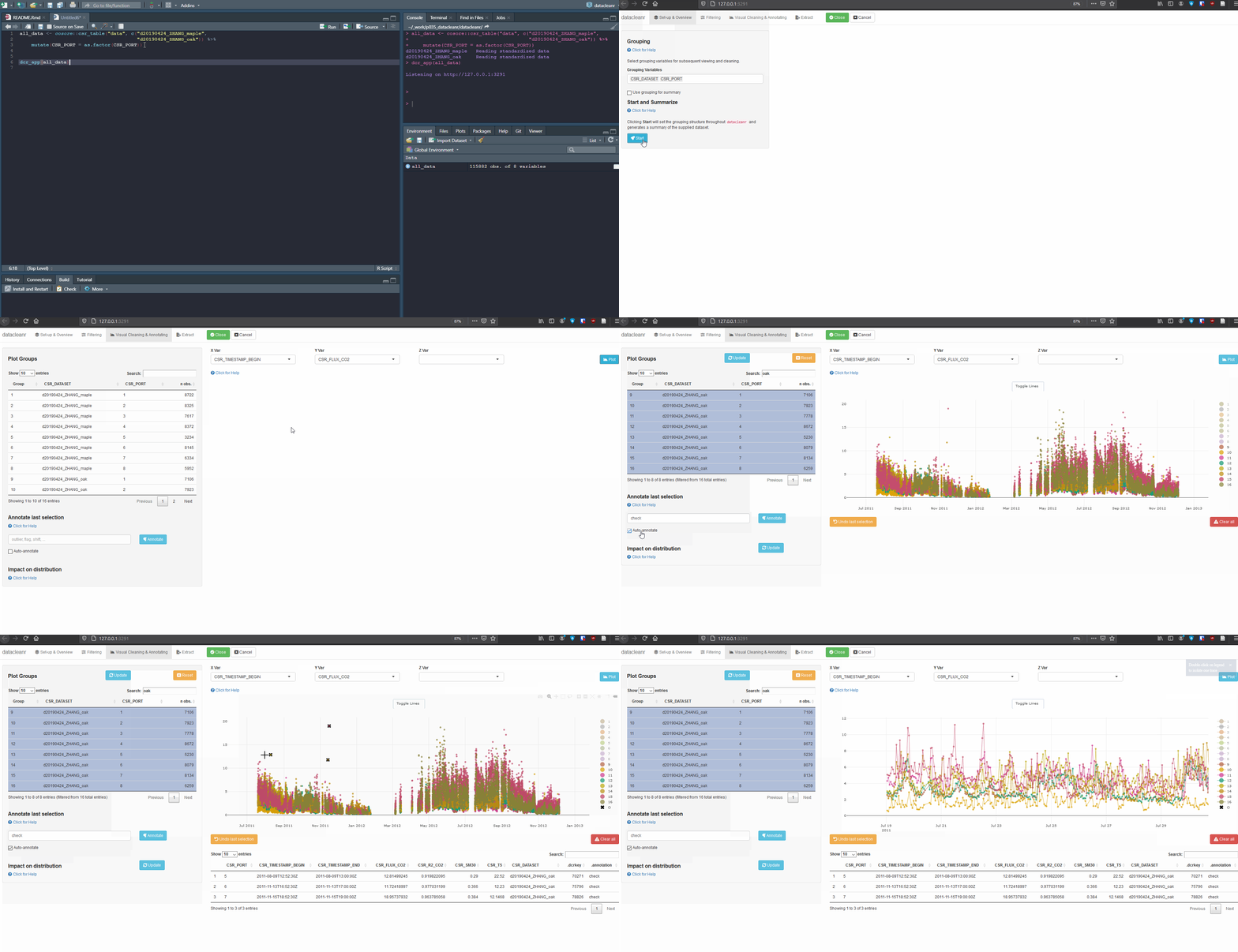
datacleanr is highly suitable for cleaning time series data, especially when comparing multiple series from similar sites or individuals (e.g. sap flow sensors in same or adjacent trees).

The example below groups soil respiration ($CO_2$ flux) from one dataset (zhang) by “sub-dataset” and measurement PORT, i.e., flux measurements in adjacent plots connected to different ports on a gas analyzer. The convenient grouping allows quick comparisons between time series, aiding in exploration and later interpretation, as well as identification of conspicuous observations:

# grab all data from ZHANG
zhang <- cosore::csr_table("data", c("d20190424_ZHANG_maple",
                                        "d20190424_ZHANG_oak")) %>%
  # adjust for grouping
  mutate(CSR_PORT = as.factor(CSR_PORT))

# group by CSR_DATASET and CSR_PORT
datacleanr::dcr_app(zhang)

7. Outlook

datacleanr is a straight-forward and powerful tool for exploring, annotating and cleaning data - this is achieved through it’s interactivity and ability to quickly cycle through (nested) groups in datasets, as well as multiple visualizations (dataset dimensions). A key component is the reproducible code that is generated to repeat any interactive steps, and hence, datacleanr can be included into any academic workflow aiming to maintain best practices in analyses.